corr

Model-implied temporal correlations of state-space model

Since R2021a

Syntax

Cyy = corr(Mdl)

Cyy = corr(Mdl,Name,Value)

[Cyy,Cxx,Cyx] = corr(___)

[Cyy,Cxx,Cyx] = corr(___,'Params',estParams)

Description

The corr function returns model-implied temporal correlations and covariances of the state or measurement variables in a stationary, time-invariant state-space model. To determine whether the model captures characteristics present in the data, You can compare model-implied associations of present and lagged variables to sample analogues. Other state-space model tools to characterize the dynamics of a specified system include the following:

• The impulse response function (IRF), computed by irf and plotted by irfplot, traces the effects of a shock to a state disturbance on the measurement variables in the system.

• The forecast error variance decomposition (FEVD), computed by fevd, provides information about the relative importance of each state disturbance in affecting the forecast error variance of all measurement variables in the system.

Fully Specified State-Space Model

Cyy = corr(Mdl) returns Corr(y_t,y_{t – 1}), the model-implied temporal correlation of each measurement variable of the fully specified, standard, stationary state-space model Mdl.

Cyy = corr(Mdl,Name,Value) uses additional options specified by one or more name-value arguments. For example, 'Covariance',true,'NumLags',10 specifies returning temporal covariances Cov(y_t,y_{t – h}), h = 0 through 10.

[Cyy,Cxx,Cyx] = corr(___) also returns Corr(x_t,x_{t – h}), the correlations between the state variables and their self-lags Cxx, and Corr(y_t,x_{t – h}), the correlations between the state variables and their self lags Cxx and the cross-correlations between the measurement variables and lags of the state variables Cyx using any of the input argument combinations in the previous syntaxes. h is the value of the NumLags name-value argument. corr returns covariances when the value of the Covariance name-value argument is true.

Partially Specified State-Space Model

[Cyy,Cxx,Cyx] = corr(___,'Params',estParams) uses the partially specified, standard state-space model Mdl and substitutes the parameter estimates estParams for all unknown parameters in the model.

Examples

Temporal Correlations of Measurement Variables

Explicitly create the state-space model

$$\begin{array}{l}{x}_{1,t}=0.9x_{1,t-1}+0.2u_{1,t}\\ x_{2,t}=0.1x_{1,t-1}+0.3x_{2,t-1}+u_{2,t}\\ y_{1,t}=x_{1,t}\\ y_{2,t}=x_{1,t}+x_{2,t}.\end{array}$$

A = [0.9 0; 0.1 0.3];
B = [0.2 0; 0 1];
C = [1 0; 1 1];
Mdl = ssm(A,B,C,'StateType',[0 0])

Mdl = 
State-space model type: ssm

State vector length: 2
Observation vector length: 2
State disturbance vector length: 2
Observation innovation vector length: 0
Sample size supported by model: Unlimited

State variables: x1, x2,...
State disturbances: u1, u2,...
Observation series: y1, y2,...
Observation innovations: e1, e2,...

State equations:
x1(t) = (0.90)x1(t-1) + (0.20)u1(t)
x2(t) = (0.10)x1(t-1) + (0.30)x2(t-1) + u2(t)

Observation equations:
y1(t) = x1(t)
y2(t) = x1(t) + x2(t)

Initial state distribution:

Initial state means
 x1  x2 
  0   0 

Initial state covariance matrix
     x1    x2   
 x1  0.21  0.03 
 x2  0.03  1.10 

State types
     x1          x2     
 Stationary  Stationary 

Mdl is an ssm model object. Because all parameters have known values, the object is fully specified.

Compute the temporal correlations of the measurement variables through lag 1.

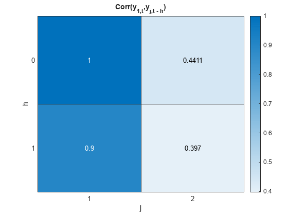
Cyy = corr(Mdl)

Cyy = 
Cyy(:,:,1) =

    1.0000    0.4411
    0.9000    0.4072


Cyy(:,:,2) =

    0.4411    1.0000
    0.3970    0.4212

Rows correspond to lags, columns correspond to the latest observation of the measurement variable in the correlation, and pages correspond to the lagged measurement variable. For example,$\mathrm{Corr}\left({\mathit{y}}_{1,\mathit{t}}{\mathit{y}}_{2,\mathit{t}-1}\right)$ is 0.3970.

Display a heatmap of the temporal correlations between the latest observation of each measurement variable and all lags of measurement variable 1.

Corryy1 = Cyy(:,:,1);
hm = heatmap(Corryy1);
ylabel('h');
hm.YDisplayLabels = ["0" "1"];
xlabel('i')
hm.XDisplayLabels = ["1" "2"];
title('Corr(y_{i,t},y_{1,t - h})')

Display a heatmap of the temporal correlations between the current observation of measurement variable 1 and all lags of all measurement variables.

Corry1y = squeeze(Cyy(:,1,:));
hm = heatmap(Corry1y);
ylabel('h');
hm.YDisplayLabels = ["0" "1"];
xlabel('j')
hm.XDisplayLabels = ["1" "2"];
title('Corr(y_{1,t},y_{j,t - h})')

Display a heatmap of the temporal correlations between the current observation of all measurement variables and the first lag of all measurement variables.

Corryylag1 = squeeze(Cyy(2,:,:));
hm = heatmap(Corryylag1);
ylabel('i');
hm.YDisplayLabels = ["1" "2"];
xlabel('j')
hm.XDisplayLabels = ["1" "2"];
title('Corr(y_{i,t},y_{j,t - 1})')

Specify Number of Periods

Explicitly create the state-space model

$$\begin{array}{l}{x}_{1,t}=0.9x_{1,t-1}+0.2u_{1,t}\\ x_{2,t}=0.1x_{1,t-1}-0.3x_{2,t-1}+u_{2,t}\\ y_{1,t}=x_{1,t}+{\epsilon }_{1,t}\\ y_{2,t}=x_{1,t}+x_{2,t}+{\epsilon }_{2,t}.\end{array}$$

A = [0.9 0; 0.1 -0.3];
B = [0.2 0; 0 1];
C = [1 0; 1 1];
D = eye(2);
Mdl = ssm(A,B,C,D,'StateType',[0 0]);

Mdl is an ssm model object.

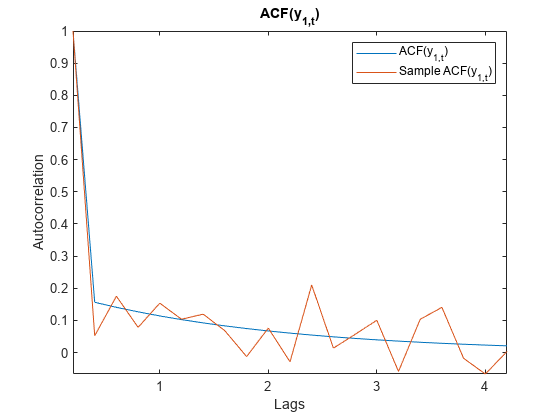
Compute the temporal correlations of the measurement variables from lag 0 through 20.

numlags = 20;
Cyy = corr(Mdl,'NumLags',numlags);

Cyy is a 21-by-2-by-2 array representing the 20-period temporal correlations of the measurement variables.

Display Cyy(:,2,2), which is the model-implied autocorrelation of ${\mathit{y}}_{2,\mathit{t}}$.

acfy2 = Cyy(:,2,2)

acfy2 = 21×1

    1.0000
   -0.0466
    0.1267
    0.0634
    0.0723
    0.0605
    0.0558
    0.0498
    0.0449
    0.0404
      ⋮

Generate a random path of measurements of length 200 from the model.

rng(1); % For reproducibility
Y = simulate(Mdl,200);

Compute the sample autocorrelation function (ACF) of each variable for 2q0 lags.

sacfy1 = autocorr(Y(:,1),'NumLags',numlags);
sacfy2 = autocorr(Y(:,2),'NumLags',numlags);

Visually compare the model-implied and sample ACF of each measurement variable.

acfy1 = Cyy(:,1,1);
plot([acfy1 sacfy1])
xticklabels(0:numlags)
ylabel("Autocorrelation")
xlabel("Lags")
legend(["ACF(y_{1,t})" "Sample ACF(y_{1,t})"])
title("ACF(y_{1,t})")
axis tight

plot([acfy2 sacfy2])
xticklabels(0:numlags)
ylabel("Autocorrelation")
xlabel("Lags")
legend(["ACF(y_{2,t})" "Sample ACF(y_{2,t})"])
title("ACF(y_{2,t})")
axis tight

State- and Cross-Variable Temporal Correlations

Explicitly create the state-space model

$$\begin{array}{l}{x}_{1,t}=0.9x_{1,t-1}+0.2u_{1,t}\\ x_{2,t}=0.1x_{1,t-1}-0.3x_{2,t-1}+u_{2,t}\\ y_{1,t}=x_{1,t}+{\epsilon }_{1,t}\\ y_{2,t}=x_{1,t}+x_{2,t}+{\epsilon }_{2,t}.\end{array}$$

A = [0.9 0; 0.1 -0.3];
B = [0.2 0; 0 1];
C = [1 0; 1 1];
D = eye(2);
Mdl = ssm(A,B,C,D,'StateType',[0 0]);

Mdl is an ssm model object.

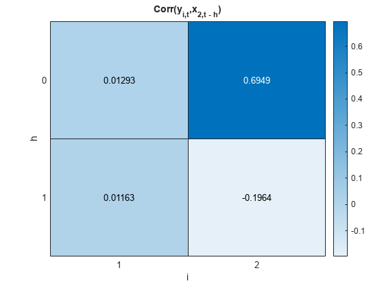
Compute the temporal correlations of the measurement and state variables, as well as their cross-correlations.

[Cyy,Cxx,Cyx] = corr(Mdl);

Each output variable is a 2-by-2-by-2 array containing temporal correlations from lag 0 to 1. Cyy contains the correlations between the measurement variables, Cxx contains the correlations among the state variables, and Cyx contains cross-correlations between the current observation of the measurement variables and lagged state variables.

Plot a heatmap of the correlations between ${\mathit{x}}_{1,\mathit{t}}$ and the lags of all state variables.

Cx1x = squeeze(Cxx(:,1,:));
hm = heatmap(Cx1x);
ylabel('h');
hm.YDisplayLabels = ["0" "1"];
xlabel('j')
hm.XDisplayLabels = ["1" "2"];
title('Corr(x_{1,t},x_{j,t - h})')

Plot a heatmap of the cross-correlations between all measurement variables and the lags of ${\mathit{x}}_{2,\mathit{t}}$.

Cyx2 = Cyx(:,:,2);
hm = heatmap(Cyx2);
ylabel('h');
hm.YDisplayLabels = ["0" "1"];
xlabel('i')
hm.XDisplayLabels = ["1" "2"];
title('Corr(y_{i,t},x_{2,t - h})')

Temporal Covariances of Estimated Model

Simulate data from a known model, fit a model to the data, and then compare sample and model-implied covariances.

Simulate Data

Explicitly create the state-space model

$$\begin{array}{l}{x}_{1,t}=0.9x_{1,t-1}+0.2u_{1,t}\\ x_{2,t}=0.1x_{1,t-1}-0.3x_{2,t-1}+u_{2,t}\\ y_{1,t}=x_{1,t}+{\epsilon }_{1,t}\\ y_{2,t}=x_{1,t}+x_{2,t}+{\epsilon }_{2,t}.\end{array}$$

ADGP = [0.9 0; 0.1 -0.3];
BDGP = [0.2 0; 0 1];
CDGP = [1 0; 1 1];
DDGP = eye(2);
DGP = ssm(ADGP,BDGP,CDGP,DDGP,'StateType',[0 0]);

Generate a random path of measurements of length 500 from the model.

rng(1); % For reproducibility
numobs = 500;
Y = simulate(DGP,numobs);

Fit Model to Data

Create a state-space model template to fit to the data by replacing each nonzero state parameter of the data-generating process with a NaN value.

A = [NaN 0; NaN NaN];
B = [NaN 0; 0 NaN];
Mdl = ssm(A,B,CDGP,DDGP,'StateType',[0  0]);

Fit the model template to the data. Specify a random set of positive starting values. Return the vector of estimated parameters.

[~,estParams] = estimate(Mdl,Y,abs(rand(5,1)));

Method: Maximum likelihood (fminunc)
Sample size: 500
Logarithmic  likelihood:     -1694.08
Akaike   info criterion:      3398.15
Bayesian info criterion:      3419.23
      |     Coeff       Std Err   t Stat     Prob  
---------------------------------------------------
 c(1) |  0.91506       0.04229   21.63956   0      
 c(2) | -0.25897       0.25406   -1.01933  0.30805 
 c(3) | -0.15383       0.08243   -1.86621  0.06201 
 c(4) | -0.16808       0.04926   -3.41221  0.00064 
 c(5) |  1.19275       0.06842   17.43153   0      
      |                                            
      |   Final State   Std Dev    t Stat    Prob  
 x(1) | -0.12293       0.30568   -0.40217  0.68756 
 x(2) | -0.80608       0.79263   -1.01697  0.30917 

Compute Covariances

Compute model-implied temporal covariances of the measurement variables by passing the state-space model template and estimated parameters to corr. Return the covariances instead of the correlations.

Covyy = corr(Mdl,'Params',estParams,'Covariance',true)

Covyy = 
Covyy(:,:,1) =

    1.1737    0.1376
    0.1589    0.1195


Covyy(:,:,2) =

    0.1376    2.5676
    0.1259   -0.1297

Covyy is a 2-by-2-by-2 array of temporal covariances of the measurement variables.

Compute the sample covariances of the measurement variables and their first lags.

AugData = lagmatrix(Y,[0 1]);
SCovyy = cov(AugData(2:end,:));

Compare Covariances

Compare the model-implied temporal covariances and the sample covariances.

names = ["y_1t" "y_2t" "y_1t-1" "y_2t-1"];

Covy1y = squeeze(Covyy(:,1,:))';
Covy2y = squeeze(Covyy(:,2,:))';
CovyLag1 = [Covy1y(:,2) Covy2y(:,2) Covy1y(:,1) Covy2y(:,1)]';
ModelCovariances = array2table([Covy1y(:) Covy2y(:) CovyLag1],'RowNames',names,...
    'VariableNames',names)

ModelCovariances=4×4 table
               y_1t        y_2t      y_1t-1      y_2t-1 
              _______    ________    _______    ________

    y_1t       1.1737     0.13759    0.15891      0.1259
    y_2t      0.13759      2.5676    0.11949    -0.12972
    y_1t-1    0.15891     0.11949     1.1737     0.13759
    y_2t-1     0.1259    -0.12972    0.13759      2.5676

SampleCovariances = array2table(SCovyy,'RowNames',names,'VariableNames',names)

SampleCovariances=4×4 table
                y_1t        y_2t       y_1t-1      y_2t-1 
              ________    ________    ________    ________

    y_1t        1.2459     0.22058     0.11689    0.070475
    y_2t       0.22058      2.5332    0.074687    -0.17466
    y_1t-1     0.11689    0.074687      1.2437     0.22158
    y_2t-1    0.070475    -0.17466     0.22158      2.5419

The model-implied and sample covariances appear to be similar in magnitude. Note that the covariances are invariant to the reference time; for example, Cov(${\mathit{y}}_{1,\mathit{t}},{\mathit{y}}_{2,\mathit{t}}$) = Cov(${\mathit{y}}_{1,\mathit{t}-1},{\mathit{y}}_{2,\mathit{t}-1}$).

Input Arguments

Mdl — Standard, stationary state-space model

ssm model object

Standard, stationary state-space model, specified as an ssm model object returned by ssm or its estimate function.

• Temporal moments are well defined for stationary states. Therefore, corr issues an error if one or more of the following conditions apply:

  • At least one state is nonstationary (Mdl.StateType contains at least one value of 2).

  • At least one coefficient is time varying.

  • Either the measurement or state variable is dimension varying.

• If Mdl is partially specified (that is, it contains unknown parameters), specify estimates of the unknown parameters by using the 'Params' name-value argument. Otherwise, corr issues an error.

• The initial covariance matrix Mdl.Cov0 is implied by the transition equation. Therefore, corr ignores Mdl.Cov0 and values corresponding to Cov0 in the value of Params.

Name-Value Arguments

Specify optional pairs of arguments as Name1=Value1,...,NameN=ValueN, where Name is the argument name and Value is the corresponding value. Name-value arguments must appear after other arguments, but the order of the pairs does not matter.

Before R2021a, use commas to separate each name and value, and enclose Name in quotes.

Example: 'Covariance',true,'NumLags',10 specifies returning Cov(y_t,y_{t – 10}), covariances of self- and cross-lags of the measurement variables from lags 0 through 10.

NumLags — Maximum number of state or measurement variable lags

1 (default) | nonnegative integer

Maximum number of state or measurement variable lags to include in the computation, specified as a nonnegative integer. corr returns associations from lags 0 through NumLags.

Example: 'NumLags',10

Data Types: double

Params — Estimates of unknown parameters

numeric vector

Estimates of the unknown parameters in the partially specified state-space model Mdl, specified as a numeric vector.

If Mdl is partially specified (contains unknown parameters specified by NaNs), you must specify Params. The estimate function returns parameter estimates of Mdl in the appropriate form. However, you can supply custom estimates by arranging the elements of Params as follows:

• If Mdl is an explicitly created model (Mdl.ParamMap is empty []), arrange the elements of Params to correspond to hits of a column-wise search of NaNs in the state-space model coefficient matrices, initial state mean vector, and covariance matrix.

  • If Mdl is time invariant, the order is A, B, C, D, Mean0, and Cov0.

  • If Mdl is time varying, the order is A{1} through A{end}, B{1} through B{end}, C{1} through C{end}, D{1} through D{end}, Mean0, and Cov0.

• If Mdl is an implicitly created model (Mdl.ParamMap is a function handle), the first input argument of the parameter-to-matrix mapping function determines the order of the elements of Params.

If Mdl is fully specified, corr ignores Params.

Example: Consider the state-space model Mdl with A = B = [NaN 0; 0 NaN] , C = [1; 1], D = 0, and initial state means of 0 with covariance eye(2). Mdl is partially specified and explicitly created. Because the model parameters contain a total of four NaNs, Params must be a 4-by-1 vector, where Params(1) is the estimate of A(1,1), Params(2) is the estimate of A(2,2), Params(3) is the estimate of B(1,1), and Params(4) is the estimate of B(2,2).

Data Types: double

Covariance — Flag for returning temporal covariances

false (default) | true

Flag for returning the temporal covariances instead of the correlations, specified as a value in this table.

Value	Description
false	Output arguments represent temporal correlations
true	Output arguments represent temporal covariances

Example: 'Covariance',true

Data Types: logical

Output Arguments

Cyy — Temporal associations of measurement variables

numeric array

Temporal associations of the measurement variables (correlations or covariances), returned as a (NumLags + 1)-by-n-by-n numeric array.

Cyy(h + 1,i,j) is the temporal association between y_i,t and y_{j,t – h}, for h = 0,1,2,...,NumLags, i = 1,2,...,n (number of measurement variables), and j = 1,2,...,n.

Cxx — Temporal associations of state variables

numeric array

Temporal associations of the state variables, returned as a (NumLags + 1)-by-m-by-m numeric array.

Cxx(h + 1,i,j) is the temporal association between x_i,t and x_{j,t – h}, for h = 0,1,2,...,NumLags, i = 1,2,...,m (number of state variables), and j = 1,2,...,m.

Cyx — Temporal cross-associations between measurement and state variables

numeric array

Temporal cross-associations between measurement and state variables, returned as a (NumLags + 1)-by-n-by-m numeric array.

Cyx(h + 1,i,j) is the temporal association between y_i,t and x_{j,t – h}, for h = 0,1,2,...,NumLags, i = 1,2,...,n, and j = 1,2,...,m.

More About

Model-Implied Temporal Associations

Model-implied temporal correlations and covariances measure self- and cross-lag associations between measurement and state variables in a state-space model, as prescribed by the model. To facilitate model specification, you can compare model-implied temporal correlations and covariances to sample analogues.

Consider the time-invariant state-space model at time t

$$\begin{array}{l}{x}_t=A{x}_{t-1}+B{u}_t\\ y_t=C{x}_t+D{\epsilon }_t.\end{array}$$

Consider a demeaned state-space model represented by state and measurement variables $${\tilde{x}}_{0,t}$$ and $${\tilde{y}}_{0,t}$$:

1. Append the state-space model with an appropriately sized constant state vector representing an intercept.

   $$\begin{array}{l}\left[\begin{array}{c}{x}_{0,t}\\ 1\end{array}\right]=\left[\begin{array}{cc}{A}_0& A_1\\ 0& 1\end{array}\right]\left[\begin{array}{c}{x}_{0,t-1}\\ 1\end{array}\right]+\left[\begin{array}{c}B\\ 0\end{array}\right]u_t\\ y_t=\left[\begin{array}{cc}{C}_0& C_1\end{array}\right]\left[\begin{array}{c}{x}_{0,t}\\ 1\end{array}\right]+D{\epsilon }_t.\end{array}$$

2. Demean the variables.

   $$\begin{array}{l}{\tilde{x}}_{0,t}=x_{0,t}-E\left(x_{0,t}\right)=x_{0,t}-{\left(I-A_0\right)}^{-1}{A}_1\\ {\tilde{y}}_{0,t}=y_{0,t}-E\left(y_{0,t}\right)=y_{0,t}-C_1-C_0{\left(I-A_0\right)}^{-1}{A}_1.\end{array}$$

3. Demean the state-space model and drop constant terms that do not affect the covariance.

   $$\begin{array}{l}{\tilde{x}}_{0,t}=A_0{\tilde{x}}_{0,t-1}+B{u}_t\\ {\tilde{y}}_{0,t}=C_0{\tilde{x}}_{0,t}+D{\epsilon }_t.\end{array}$$

Because the difference between the full state-space model and the demeaned model is the inclusion of constant states, $$\text{Cov}(x_t,x_{t-h})=\text{Cov}\left({\tilde{x}}_{0,t},{\tilde{x}}_{0,t-h}\right)={\Gamma }_{0,h},$$ which implies

$$Cxx(1,:,:)={\Gamma }_{0,0}=A_0{\Gamma }_{0,0}{A}_0\prime +BB\prime .$$

Let $${\tilde{\Gamma }}_{0,0}$$ be the solution to the equation. Using the demeaned state equation,

$$Cxx(h+1,:,:)={\Gamma }_{0,h}=A_o{\Gamma }_{h-1};h=1,2,\mathrm{....}$$

The preceding results imply the following:

• $$Cyy(1,:,:)=\text{Cov}\left(y_t,y_t\right)=C_0{\Gamma }_{0,0}{C}_0^{\prime }+D{D}^{\prime }.$$

• $$Cyy(h+1,:,:)=\text{Cov}\left(y_t,y_{t-h}\right)=C_0{\Gamma }_{0,h}{C}_0^{\prime };h=1,2,\mathrm{....}$$

• $$Cyx(h+1:,:)=\text{Cov}(y_t,x_{t-h})=C_0{\Gamma }_{0,h};h=0,1,\mathrm{2....}$$

Tips

• To obtain an association matrix of lead variables from an association matrix of lagged variables, use the identity

  $$C\left(a_t,b_{t+h}\right)=C{\left(a_t,b_{t-h}\right)}^{\prime },$$

  where:

  • C is an association function, either Corr or Cov.

  • a_t and b_t are y_t or x_t.

Version History

Introduced in R2021a