Simulate Responses of Estimated VARX Model
This example shows how to estimate a multivariate time series model that contains lagged endogenous and exogenous variables, and how to simulate responses. The response series are the quarterly:
Changes in real gross domestic product (rGDP) rates ()
Real money supply (rM1SL) rates ()
Short-term interest rates (i.e., three-month treasury bill yield, )
from March, 1959 through March, 2009. The exogenous series is the quarterly changes in the unemployment rates ().
Suppose that a model for the responses is this VARX(4,3) model
Preprocess the Data
Load the U.S. macroeconomic data set. Flag the series and their periods that contain missing values (indicated by NaN values).
load Data_USEconModel
varNaN = any(ismissing(DataTimeTable),1); % Variables containing NaN values
seriesWithNaNs = series(varNaN)
seriesWithNaNs = 1×5 cell
    {'(FEDFUNDS) Effective federal funds rate'}    {'(GS10) Ten-year treasury bond yield'}    {'(M1SL) M1 money supply (narrow money)'}    {'(M2SL) M2 money supply (broad money)'}    {'(UNRATE) Unemployment rate'}
In this data set, the variables that contain missing values entered the sample later than the other variables. There are no missing values after sampling started for a particular variable.
Flag all periods corresponding to missing values in the model variables.
idx = all(~ismissing(DataTimeTable(:,{'UNRATE' 'M1SL'})),2);For the rest of the example, consider only those values that of the series indicated by a true in idx.
Compute rGDP and rM1SL, and the growth rates of rGDP, rM1SL, short-term interest rates, and the unemployment rate. Description contains a description of the data and the variable names. Reserve the last three years of data to investigate the out-of-sample performance of the estimated model.
rGDP = DataTimeTable.GDP(idx)./(DataTimeTable.GDPDEF(idx)/100);
rM1SL = DataTimeTable.M1SL(idx)./(DataTimeTable.GDPDEF(idx)/100);

dLRGDP = diff(log(rGDP));              % rGDP growth rate
dLRM1SL = diff(log(rM1SL));            % rM1SL growth rate
d3MTB = diff(DataTimeTable.TB3MS(idx));    % Change in short-term interest rate (3MTB)
dUNRATE = diff(DataTimeTable.UNRATE(idx)); % Change in unemployment rate

T = numel(d3MTB);    % Total sample size
oosT = 12;           % Out-of-sample size
estT = T - oosT;     % Estimation sample size
estIdx = 1:estT;     % Estimation sample indices
oosIdx = (T - 11):T; % Out-of-sample indices
dt = DataTimeTable.Time;
dt = dt((end - T + 1):end);

EstY = [dLRGDP(estIdx) dLRM1SL(estIdx) d3MTB(estIdx)]; % In-sample responses
estX = dUNRATE(estIdx);                                % In-sample exogenous data
n = size(EstY,2);

OOSY = [dLRGDP(oosIdx) dLRM1SL(oosIdx) d3MTB(oosIdx)]; % Out-of-sample responses
oosX = dUNRATE(oosIdx);                                % Out-of-sample exogenous data
Create VARX Model
Create a VARX(4) model using varm.
Mdl = varm(n,4);
Mdl is a varm model object serving as a template for estimation. Currently, Mdl does know have the structure in place for the regression component. However, MATLAB® creates the required structure during estimation.
Estimate the VAR(4) Model
Estimate the parameters of the VARX(4) model using estimate. Display the parameter estimates.
EstMdl = estimate(Mdl,EstY,'X',estX);
summarize(EstMdl)
   AR-Stationary 3-Dimensional VARX(4) Model with 1 Predictor

    Effective Sample Size: 184
    Number of Estimated Parameters: 42
    LogLikelihood: 1037.52
    AIC: -1991.04
    BIC: -1856.01

                      Value       StandardError    TStatistic      PValue
                   ___________    _____________    __________    __________

    Constant(1)      0.0080266     0.00097087         8.2674     1.3688e-16
    Constant(2)     0.00063838      0.0015942        0.40044        0.68883
    Constant(3)       0.068361          0.143        0.47803        0.63263
    AR{1}(1,1)       -0.034045        0.06633       -0.51327        0.60776
    AR{1}(2,1)      -0.0024555        0.10891      -0.022546        0.98201
    AR{1}(3,1)         -1.7163           9.77       -0.17567        0.86056
    AR{1}(1,2)       -0.013882       0.046481       -0.29867        0.76519
    AR{1}(2,2)         0.17753       0.076323          2.326       0.020017
    AR{1}(3,2)         -6.7572         6.8464       -0.98697        0.32366
    AR{1}(1,3)       0.0010682     0.00048092         2.2212       0.026337
    AR{1}(2,3)      -0.0050252     0.00078967        -6.3636     1.9705e-10
    AR{1}(3,3)        -0.16256       0.070837        -2.2948       0.021744
    AR{2}(1,1)        0.077748       0.064014         1.2145        0.22454
    AR{2}(2,1)       0.0047257        0.10511       0.044959        0.96414
    AR{2}(3,1)          3.4244         9.4289        0.36318        0.71647
    AR{2}(1,2)        0.077867       0.046954         1.6584       0.097245
    AR{2}(2,2)         0.29087       0.077099         3.7727     0.00016148
    AR{2}(3,2)         0.39284         6.9161         0.0568         0.9547
    AR{2}(1,3)      -0.0010719     0.00056413        -1.9001       0.057423
    AR{2}(2,3)      -0.0016135     0.00092631        -1.7419       0.081533
    AR{2}(3,3)        -0.21556       0.083094        -2.5942      0.0094802
    AR{3}(1,1)       -0.090881       0.062563        -1.4526        0.14633
    AR{3}(2,1)        0.064249        0.10273        0.62542        0.53169
    AR{3}(3,1)         -7.9727         9.2152       -0.86517        0.38695
    AR{3}(1,2)       -0.024092        0.04631       -0.52024        0.60289
    AR{3}(2,2)        0.068565       0.076041        0.90168        0.36723
    AR{3}(3,2)          10.263         6.8212         1.5046        0.13242
    AR{3}(1,3)     -0.00055981     0.00056073       -0.99836        0.31811
    AR{3}(2,3)      -0.0021302     0.00092073        -2.3136        0.02069
    AR{3}(3,3)         0.22969       0.082593         2.7809      0.0054203
    AR{4}(1,1)        0.066151       0.056841         1.1638        0.24451
    AR{4}(2,1)        0.028826       0.093334        0.30885        0.75744
    AR{4}(3,1)          1.0379         8.3724        0.12397        0.90134
    AR{4}(1,2)       -0.078735       0.043804        -1.7975       0.072263
    AR{4}(2,2)       0.0096425       0.071926        0.13406        0.89335
    AR{4}(3,2)         -12.007         6.4521        -1.8609       0.062761
    AR{4}(1,3)     -0.00018454     0.00053356       -0.34586        0.72945
    AR{4}(2,3)     -0.00019036     0.00087611       -0.21728        0.82799
    AR{4}(3,3)        0.053812       0.078591        0.68471        0.49353
    Beta(1,1)        -0.016084      0.0016037        -10.029     1.1365e-23
    Beta(2,1)         -0.00154      0.0026333       -0.58482        0.55867
    Beta(3,1)          -1.5317        0.23622        -6.4841     8.9252e-11


   Innovations Covariance Matrix:
    0.0000    0.0000    0.0000
    0.0000    0.0001   -0.0019
    0.0000   -0.0019    0.7790


   Innovations Correlation Matrix:
    1.0000    0.1198    0.0011
    0.1198    1.0000   -0.2177
    0.0011   -0.2177    1.0000
EstMdl is a varm model object containing the estimated parameters.
Simulate Out-Of-Sample Response Paths
Simulate 1000, 3 year response series paths from the estimated model assuming that the exogenous unemployment rate is a fixed series. Since the model contains 4 lags per endogenous variable, specify the last 4 observations in the estimation sample as presample data.
numPaths = 1000;
Y0 = EstY((end-3):end,:);
rng(1); % For reproducibility
YSim = simulate(EstMdl,oosT,'X',oosX,'Y0',Y0,'NumPaths',numPaths);
YSim is a 12-by-3-by-1000 numeric array of simulated responses. The rows of YSim correspond to out-of-sample periods, the columns correspond to the response series, and the pages correspond to paths.
Plot the response data and the simulated responses. Identify the 5%, 25%, 75% and 95% percentiles, and the mean and median of the simulated series at each out-of-sample period.
YSimBar = mean(YSim,3);
YSimQrtl = quantile(YSim,[0.05 0.25 0.5 0.75 0.95],3);
respNames = {'dLRGDP' 'dLRM1SL' 'd3MTB'};

figure;
for j = 1:n
    subplot(3,1,j);
    h1 = plot(dt(oosIdx),squeeze(YSim(:,j,:)),'Color',0.75*ones(3,1));
    hold on
    h2 = plot(dt(oosIdx),YSimBar(:,j),'.-k','LineWidth',2);
    h3 = plot(dt(oosIdx),squeeze(YSimQrtl(:,j,:)),':r','LineWidth',1.5);
    h4 = plot(dt((end - 30):end),[EstY((end - 18):end,j);OOSY(:,j)],...
        'b','LineWidth',2);
    title(sprintf('%s',respNames{j}));
    axis tight
    hold off
end
legend([h1(1) h2(1) h3(1) h4],{'Simulated Series','Simulation Mean',...
    'Simulation Quartile','Data'},'Location',[0.4 0.1 0.01 0.01],...
    'FontSize',8);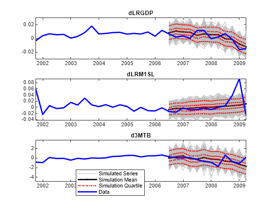
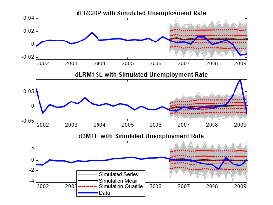
Simulate Out-Of-Sample Response Paths Using Random Exogenous Data
Suppose that the change in the unemployment rate is an AR(4) model, and fit the model to the estimation sample data.
MdlUNRATE = arima('ARLags',1:4);
EstMdlUNRATE = estimate(MdlUNRATE,estX,'Display','off');
EstMdlUNRATE is an arima model object containing the parameter estimates.
Simulate 1000, 3 year paths from the estimated AR(4) model for the change in unemployment rate. Since the model contains 4 lags, specify the last 4 observations in the estimation sample as presample data.
XSim = simulate(EstMdlUNRATE,oosT,'Y0',estX(end-3:end),...
    'NumPaths',numPaths);
XSim is a 12-by-1000 numeric matrix of simulated exogenous paths. The rows correspond to periods and the columns correspond to paths.
Simulate 3 years of 1000 future response series paths from the estimated model using the simulated exogenous data. simulate does not accept multiple paths of predictor data, so you must simulate responses in a loop. Since the model contains 4 lags per endogenous variable, specify the last 4 observations in the estimation sample as presample data.
YSimRX = zeros(oosT,n,numPaths); % Preallocate

for j = 1:numPaths
    YSimRX(:,:,j) = simulate(EstMdl,oosT,'X',XSim(:,j),'Y0',Y0);
end
YSimRX is a 12-by-3-by-1000 numeric array of simulated responses.
Plot the response data and the simulated responses. Identify the 5%, 25%, 75% and 95% percentiles, and the mean and median of the simulated series at each out-of-sample period.
YSimBarRX = mean(YSimRX,3);
YSimQrtlRX = quantile(YSimRX,[0.05 0.25 0.5 0.75 0.95],3);

figure;
for j = 1:n
    subplot(3,1,j);
    h1 = plot(dt(oosIdx),squeeze(YSimRX(:,j,:)),'Color',0.75*ones(3,1));
    hold on
    h2 = plot(dt(oosIdx),YSimBarRX(:,j),'.-k','LineWidth',2);
    h3 = plot(dt(oosIdx),squeeze(YSimQrtlRX(:,j,:)),':r','LineWidth',1.5);
    h4 = plot(dt((end - 30):end),[EstY((end - 18):end,j);OOSY(:,j)],...
        'b','LineWidth',2);
    title(sprintf('%s with Simulated Unemployment Rate Change',respNames{j}));
    axis tight
    hold off
end
legend([h1(1) h2(1) h3(1) h4],{'Simulated Series','Simulation Mean',...
    'Simulation Quartile','Data'},'Location',[0.4 0.1 0.01 0.01],...
    'FontSize',8)