recreg
Recursive linear regression
Syntax
Description
recreg recursively estimates coefficients
(β) and their standard errors in a multiple linear regression
model of the form y = Xβ + ε by
performing successive regressions using nested or rolling windows.
recreg has options for OLS, HAC, and FGLS estimates, and
for iterative plots of the estimates.
[
returns a table of regression coefficients estimates and a table of standard
error estimates from a recursive regression on the linear model of the
variables in the input table or timetable.CoeffTbl,SETbl] = recreg(Tbl)
The response variable in the regression is the last table variable, and all
other variables are the predictor variables. To select a different response
variable for the regression, use the ResponseVariable
name-value argument. To select different predictor variables, use the
PredictorNames name-value argument.
___ = recreg(___,
specifies options using one or more name-value arguments in
addition to any of the input argument combinations in previous syntaxes.
Name=Value)recreg returns the output argument combination for the
corresponding input arguments. For example,
recreg(Tbl,ResponseVariable="GDP",Intercept=false,Estimator="fgls")
excludes an intercept term from the regression model, in which the response
variable is the variable GDP in the input table, and uses
FGLS to estimate coefficients and standard errors.
recreg(___) plots iterative coefficient
estimates with ±2 standard error bands for each coefficient in the multiple
linear regression model.
___ = recreg(
plots on the axes specified in ax,___)ax instead of the axes of new
figures. The option ax can precede any of the input argument
combinations in the previous syntaxes.
[___,
additionally returns handles to plotted graphics objects. Use elements of
coeffPlots] = recreg(___)coeffPlots to modify properties of the plots after you
create it.
Examples
Check coefficient estimates for instability in a model of food demand around World War II. Implement forward and backward recursive regressions in a rolling window.
Load the US food consumption data set, which contains annual measurements from 1927 through 1962 with missing data due to WWII.
load Data_ConsumptionFor more details on the data, enter Description at the command prompt.
Plot the series.
P = Data(:,1); % Food price index
I = Data(:,2); % Disposable income index
Q = Data(:,3); % Food consumption index

figure
plot(dates,[P I Q])
axis tight
grid on
xlabel("Year")
ylabel("Index")
title("\bf Time Series Plot of All Series")
legend("Price","Income","Consumption",Location="southeast")
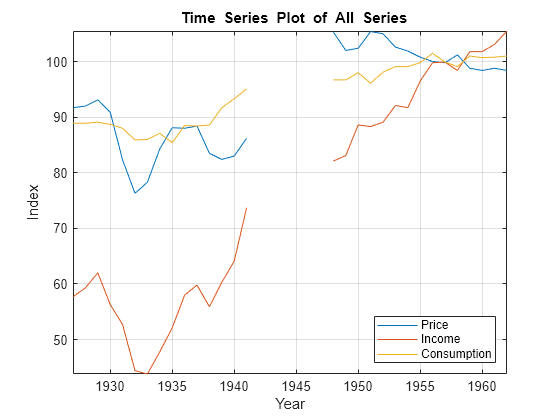
Measurements are missing from 1942 through 1947, which correspond to WWII.
To examine elasticities, apply the log transformation to each series.
LP = log(P);
LI = log(I);
LQ = log(Q);
Consider a model in which log consumption is a linear function of the logs of food price and income. In other words,
is a Gaussian random variable with mean 0 and standard deviation .
Identify the breakpoint index at the end of WWII, 1945. Ignore missing years with missing data.
numCoeff = 4; % Three predictors and an intercept
T = numel(dates(~isnan(P))); % Sample size
bpIdx = find(dates(~isnan(P)) >= 1945,1) - numCoeff
bpIdx =
12
The 12th iteration corresponds to the end of the war.
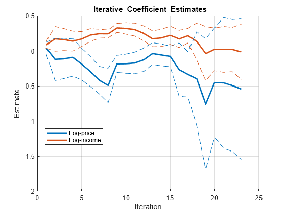
Plot forward recursive-regression coefficient estimates using a rolling window 1/4 of the sample size. Indicate to plot the coefficients of LP and LI only in the same figure.
X = [LP LI];
y = LQ;
varnames = ["Log-price" "Log-income"];
plotvars = [false true true];
window = ceil(T*1/4);
recreg(X,y,Window=window,Plot="combined",PlotVars=plotvars, ...
    VarNames=varnames);
Plot forward recursive-regression coefficient estimates using a rolling window 1/3 of the sample size.
window = ceil(T*1/3);
recreg(X,y,Window=window,Plot="combined",PlotVars=plotvars, ...
    VarNames=varnames);

Plot forward recursive-regression coefficient estimates using a rolling window of size 1/2 of the sample size.
window = ceil(T*1/2);
recreg(X,y,Window=window,Plot="combined",PlotVars=plotvars, ...
    VarNames=varnames);
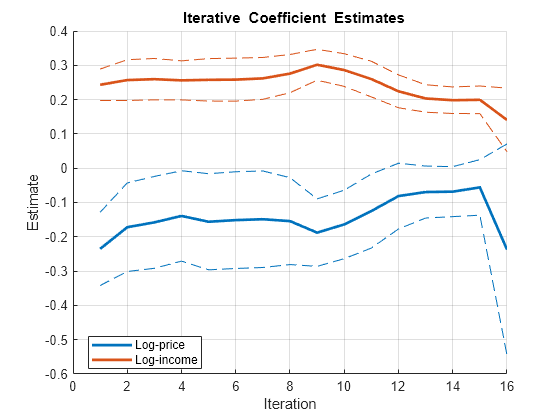
As the window size increases, the lines show less volatility, but the coefficients do exhibit instability.
Apply recursive regressions using nested windows to look for instability in an explanatory model of real GNP for a period spanning World War II.
Load the Nelson-Plosser data set.
load Data_NelsonPlosserThe time series in the data set contain annual, macroeconomic measurements from 1860 to 1970. For more details, a list of variables, and descriptions, enter Description in the command line.
Several series have missing data. Focus the sample to measurements from 1915 to 1970. Identify the index corresponding to 1945, the end of WWII, to use as a breakpoint for the test.
span = (1915 <= dates) & (dates <= 1970);
bp = find(dates(span) == 1945);
Consider the multiple linear regression model
Collect the model variables into a tabular array. Position the predictors in the first three columns and the response in the last column. Compute the number of coefficients in the model.
Tbl = DataTable(span,[4,5,10,1]);
numCoeff = height(Tbl);
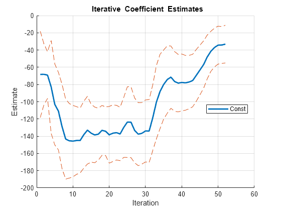
Estimate the coefficients using recursive regressions, and return separate plots for the iterative estimates. Identify the iteration corresponding to the end of the war.
recreg(Tbl);
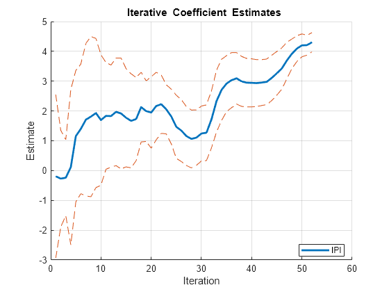
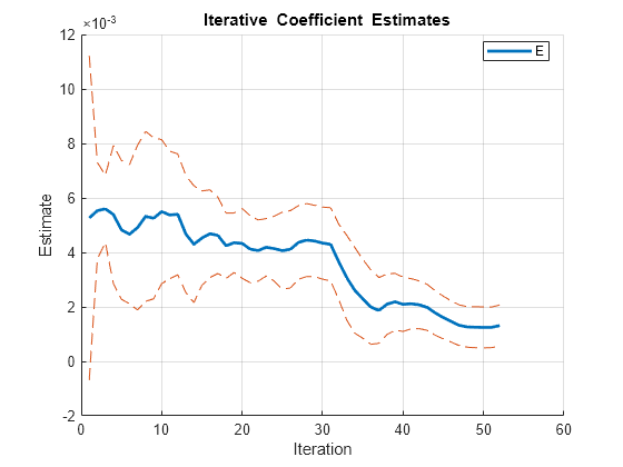
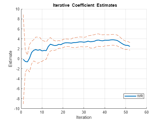
bpIter = bp - numCoeff
bpIter =
-25
By default, recreg forms the subsamples using nested windows. The end of the war (1945) occurs at the 27th iteration.
All coefficients show some initial, transient instability during the "burn-in" period (see Tip). The plot of WR seems stable since the line is relatively flat. However, the plots of E, IPI, and the intercept (Const) show instability, particularly just after iteration 27.
Return tables of iterative coefficient estimates and a table of standard errors.
[CoeffTbl,SeTbl] = recreg(Tbl)
CoeffTbl=4×52 table
               Iter1        Iter2        Iter3        Iter4        Iter5        Iter6        Iter7        Iter8       Iter9       Iter10       Iter11       Iter12       Iter13       Iter14       Iter15       Iter16       Iter17       Iter18       Iter19       Iter20       Iter21       Iter22       Iter23       Iter24       Iter25       Iter26       Iter27       Iter28       Iter29       Iter30       Iter31       Iter32       Iter33       Iter34       Iter35       Iter36       Iter37       Iter38       Iter39       Iter40      Iter41       Iter42       Iter43       Iter44       Iter45       Iter46       Iter47       Iter48      Iter49       Iter50       Iter51       Iter52
             _________    _________    _________    _________    _________    _________    _________    _________    ________    _________    _________    _________    _________    _________    _________    _________    _________    _________    _________    _________    _________    _________    _________    _________    _________    _________    _________    _________    _________    _________    _________    _________    _________    _________    _________    _________    _________    _________    _________    ________    _________    _________    _________    _________    _________    _________    _________    ________    _________    _________    _________    _________

    Const      -68.313      -68.159       -69.09      -82.751      -103.08      -110.89      -128.78      -143.35     -145.34       -145.7      -144.99      -144.89      -138.22      -132.97      -136.44       -138.5      -137.67      -133.23      -134.23       -138.4      -136.51      -135.89       -137.4      -129.78      -123.62      -123.76      -133.27      -137.67      -136.66       -133.9      -134.03      -118.43      -100.44      -88.055      -79.962       -74.23      -71.441      -76.452      -78.424     -77.625      -78.071      -77.155      -75.387      -69.307      -63.127      -56.891      -48.067     -41.498      -37.059      -34.289      -34.159      -33.111
    IPI       -0.19396     -0.26934     -0.23743       0.1147       1.1563       1.4004       1.7091       1.8108      1.9295       1.6962       1.8353       1.8286       1.9712       1.9167       1.7732       1.6692       1.7286       2.1302        1.995       1.9489       2.1656       2.2272       2.0554       1.8136       1.4672       1.3415       1.1593       1.0618       1.1066       1.2453       1.2701       1.7212       2.3317       2.7073       2.9193       3.0347       3.0946       2.9913       2.9503      2.9431       2.9357       2.9536       2.9781       3.1112       3.2635       3.4263       3.6943      3.9185       4.0934       4.2018        4.208       4.3063
    E        0.0052645    0.0055309    0.0055981    0.0053891    0.0048281    0.0046665    0.0049113    0.0053202    0.005254    0.0054972    0.0053744    0.0053981    0.0046767    0.0043011    0.0045254    0.0046878    0.0046215    0.0042438    0.0043549    0.0043299    0.0041189    0.0040688    0.0041893    0.0041366    0.0040636    0.0041145    0.0043661    0.0044527    0.0044182    0.0043419    0.0042948    0.0036566    0.0030707    0.0026066    0.0022932    0.0019903    0.0018696    0.0020991    0.0021872    0.002095    0.0021159    0.0020759    0.0019813    0.0017761    0.0016083    0.0014596    0.0013216    0.001264    0.0012525    0.0012474    0.0012488    0.0013136
    WR         -0.1097     -0.52635     -0.62228      0.10675       1.2592       1.7072       1.8568       1.7174      1.8357        1.591       1.6799       1.6407       2.4802       2.9305       2.7864        2.664       2.7035       2.8985       2.8403       3.0737        3.208       3.2268       3.1978       3.1503       3.2559       3.2607       3.3254       3.4107       3.4009       3.3355       3.3988       3.5459        3.427       3.4651       3.5263       3.7157       3.7646       3.6554        3.616      3.7333       3.7218       3.7393       3.8059       3.8214       3.7642       3.6691       3.4004      3.1159        2.866       2.7074       2.6967       2.4962
SeTbl=4×52 table
               Iter1        Iter2         Iter3        Iter4        Iter5        Iter6        Iter7       Iter8       Iter9       Iter10       Iter11       Iter12       Iter13      Iter14        Iter15        Iter16        Iter17        Iter18        Iter19        Iter20        Iter21        Iter22        Iter23        Iter24       Iter25        Iter26        Iter27        Iter28        Iter29        Iter30        Iter31        Iter32        Iter33        Iter34        Iter35        Iter36        Iter37        Iter38       Iter39        Iter40        Iter41       Iter42       Iter43       Iter44      Iter45       Iter46        Iter47        Iter48        Iter49        Iter50        Iter51        Iter52
             _________    __________    __________    ________    _________    _________    _________    _______    _________    _________    _________    _________    ________    _________    __________    __________    __________    __________    __________    __________    __________    __________    __________    __________    _________    __________    __________    __________    __________    __________    __________    __________    __________    __________    __________    __________    __________    __________    _________    __________    __________    ________    __________    ________    ________    __________    __________    __________    __________    __________    __________    __________

    Const       25.046        17.761        13.542      26.937       23.487        22.49       24.476      23.21       21.624       20.733       19.635       18.804      19.415       19.645        16.837        16.147        15.053        14.482        14.056         16.46        16.437        15.861         15.51        17.403       20.502        20.579        18.795        18.287        17.856         17.98        18.278        19.066        21.269        21.564         20.02        19.564        18.059        17.337       16.675         16.51        15.886      15.449        15.237      15.021      14.431        13.733        12.725          11.6        11.285         10.99        10.724        10.927
    IPI          1.372        0.8095       0.63806      1.3034       1.1015       1.0866       1.2787     1.3444       1.2505       1.0933      0.89532      0.85677      0.9022      0.93004       0.82359       0.78861       0.69814        0.5849       0.50843       0.59812       0.56616       0.48889       0.41153       0.45871      0.52933       0.51865       0.49419       0.48475       0.46515       0.45985       0.46714       0.47995       0.51801        0.5138       0.46896       0.46184        0.4317       0.41892      0.40603       0.40296       0.39324     0.38492       0.38225      0.3798     0.36581       0.34681       0.30661       0.24728       0.21661       0.19106       0.16727       0.16107
    E        0.0029773    0.00088806    0.00061649    0.001268    0.0012745    0.0012768    0.0015111    0.00156    0.0014781    0.0013213    0.0011703    0.0011097    0.001074    0.0010721    0.00086491    0.00080439    0.00069756    0.00059868    0.00054492    0.00064127    0.00061363    0.00056167    0.00052574    0.00059848    0.0007086    0.00070974    0.00067556    0.00067026    0.00065521    0.00066166    0.00067179    0.00069178    0.00077754    0.00078678    0.00072299    0.00068182    0.00060376    0.00055766    0.0005213    0.00049814    0.00046066    0.000438    0.00042075    0.000408    0.000392    0.00037819    0.00037353    0.00037249    0.00037624    0.00037665    0.00037242    0.00037821
    WR          4.4923        1.0841       0.69505      1.3781       1.1311       1.0576       1.2544     1.3167       1.2237       1.0535      0.94646      0.86648     0.73106      0.67509       0.53986       0.48929       0.42646       0.38471       0.35942       0.41265       0.39531        0.3785       0.37151       0.42274      0.49945       0.50132       0.50008       0.49299       0.48526        0.4894       0.49548       0.54059       0.62494       0.65764       0.65499       0.63966       0.62063       0.61069      0.59915       0.56739       0.55232     0.54357       0.53533     0.54476     0.54798       0.54741       0.52804       0.47669       0.44754        0.4222       0.38934       0.38022
If a linear regression model violates classical linear model assumptions, then OLS coefficient standard errors are incorrect. However, recreg has options to estimate coefficients and standard errors that are robust to heteroscedastic or autocorrelated innovations.
Simulate a series from this piecewise regression model with AR(1) errors whose regression coefficient changes at time 51.
is a series of Gaussian innovations with mean 0 and standard deviation 0.5. is Gaussian with mean 1 and standard deviation 0.25.
rng(1); % For reproducibility
T = 100;
muX = 1;
sigmaX = 0.25;
x = sigmaX*randn(T,1) + muX;
ar = 0.6;
sigma = 0.5;
c = 5;
b = [3 -1];
y = zeros(T,1);
Mdl1 = regARIMA(AR=ar,Variance=sigma,Intercept=c,Beta=b(1));
y(1:T/2) = simulate(Mdl1,T/2,X=x(1:T/2));
Mdl2 = regARIMA(AR=ar,Variance=sigma,Intercept=c,Beta=b(2));
y((T/2 + 1):T) = simulate(Mdl2,T/2,X=x((T/2 + 1):T));
Estimate recursive regression coefficients using OLS.
[CoeffOLS,SEOLS] = recreg(x,y,Plot="separate");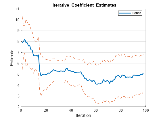
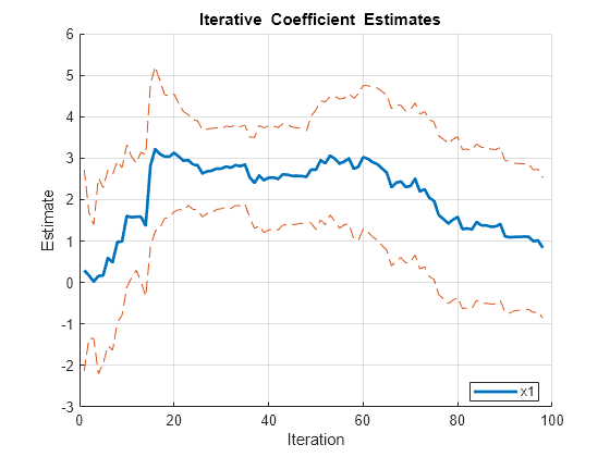
After transient effects, 5 is within the confidence bounds of the intercept estimates. There is an insignificant but persistent shock at iteration 50. The coefficient estimates show the structural change after iteration 60.
To account for autocorrelated innovations, estimate recursive regression coefficients using OLS, but with Newey-West robust standard errors. For estimating the HAC standard errors, use the quadratic-spectral weighting scheme.
hacOptions.Weights = "QS"hacOptions = struct with fields:
Weights: "QS"
[CoeffNW,SENW] = recreg(x,y,Estimator="hac",Options=hacOptions, ...
    Plot="separate");
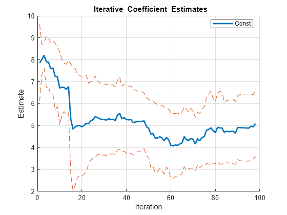
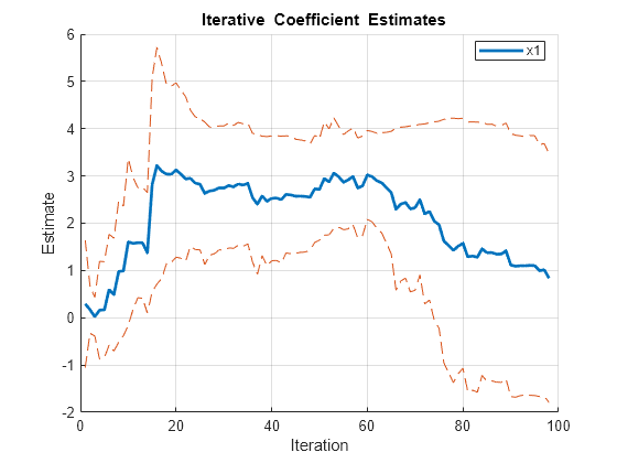
The HAC coefficient estimates are the same as the OLS estimates. The confidence bounds are slightly different because the standard error estimators are different.
Input Arguments
Predictor data X for the multiple linear regression model,
specified as a numObs-by-numPreds numeric
matrix.
Each row represents one of the numObs observations and each column
represents one of the numPreds predictor variables.
Data Types: double
Response data y for the multiple linear
regression model, specified as a
numObs-by-1 numeric vector.
Rows of y and
X correspond.
Data Types: double
Combined predictor and response data for the multiple linear regression model,
specified as a table or timetable with numObs rows. Each row of
Tbl is an observation.
The test regresses the response variable, which is the last variable in
Tbl, on the predictor variables, which are all other variables
in Tbl. To select a different response variable for the regression,
use the ResponseVariable name-value argument. To select different
predictor variables, use the PredictorNames name-value argument to
select numPreds predictors.
Note
NaNs in X,
y, or Tbl indicate missing values, and
recreg removes observations containing at least one
NaN. That is, to remove NaNs in X
or y, recreg merges the variables [X
y], and then it uses list-wise deletion to remove any row that contains at least
one NaN. recreg also removes any row of
Tbl containing at least one NaN. Removing
NaNs in the data reduces the sample size and can create irregular time
series.
Name-Value Arguments
Specify optional pairs of arguments as
Name1=Value1,...,NameN=ValueN, where Name is
the argument name and Value is the corresponding value.
Name-value arguments must appear after other arguments, but the order of the
pairs does not matter.
Before R2021a, use commas to separate each name and value, and enclose
Name in quotes.
Example: recreg(Tbl,ResponseVariable="GDP",Intercept=false,Estimator="fgls")
excludes an intercept term from the regression model, in which the response variable
is the variable GDP in the table Tbl, and
uses FGLS to estimate coefficients and standard errors.
Flag to include a model intercept, specified as a value in this table.
| Value | Description |
|---|---|
true | recreg includes an intercept term in the regression model. numCoeffs = numPreds + 1. |
false | recreg does not include an intercept when fitting the regression model. numCoeffs = numPreds. |
Example: Intercept=false
Data Types: logical
Window length, specified as a numeric scalar.
To compute estimates using nested windows, do not specify
Window. In this case,recregbegins with the firstnumCoeffs+ 1 observations, and then adds one observation at each iteration. The number of iterations isnumIter=numObs–numCoeffs.To compute estimates using a rolling window, specify a window length. In this case,
recregshifts by one observation at each iteration.Windowmust be at leastnumCoeffs+ 1 and at mostnumObs. The number of iterations isnumIter=numObs–Window+ 1.
Example: Window=10
Data Types: double
Estimation method, specified as a value in this table.
| Value | Description |
|---|---|
"ols" | Ordinary least squares |
"hac" | Heteroscedasticity and autocorrelation consistent (HAC) standard errors |
"fgls" | Feasible generalized least squares coefficients and standard errors |
Values "hac" and "fgls" call
hac and fgls, respectively, with
optional name-value arguments specified by
Options.
Example: Estimator="fgls"
Data Types: char | string
hac and fgls optional name-value
argument names and corresponding values, specified as a structure
scalar.
Use Options to set any name-value argument except
VarNames, Intercept,
Display, Plot,
ResponseVariable, and
PredictorVariables. For these options, see
corresponding recreg name-value
arguments.
By default, recreg calls
hac or fgls using
defaults. If Estimator="ols",
recreg ignores
Options.
Example: Options=struct("ARLags",2) includes two
lags in the AR innovations model for FGLS estimators.
Data Types: struct
Iteration direction, specified as a value in this table.
| Value | Description |
|---|---|
"forward" | Forward recursions move the window of observations from the beginning of the data to the end. |
"backward" | Backward recursions first reverse the order of observations, and then implement forward recursions. |
Example: Direction="backward"
Data Types: char | string
Coefficient estimate plot control, specified as a value in this table. Plots show iterative coefficient estimates with ±2 standard error bands.
| Value | Description |
|---|---|
"separate" | recreg produces
separate figures for each coefficient. |
"combined" | recreg combines all
plots in a single set of axes. |
"off" | recreg turns off all
plotting. |
The defaults are:
"off"whenrecregreturns output arguments"separate"otherwise
Example: Plot=off
Data Types: char | string
Flags for which coefficients to plot, specified as a logical vector of
length numCoeffs. The first element corresponds to
Intercept, if present, followed by indicators
for each of the numPred predictors in
X or Tbl. The default is
true(numCoeffs,1) to plot all
coefficients.
Example: PlotVars=[false true true false] plots the
second and third coefficients of four coefficients.
Data Types: logical
Variable names for plotted coefficients, specified as a string vector
or cell vector of strings of a length numCoeffs:
If
Intercept=true,VarNames(1)is the name of the intercept (for example'Const') andVarNames(specifies the name to use for variablej+ 1)X(:,orj)PredictorVariables(.j)If
Intercept=false,VarNames(specifies the name to use for variablej)X(:,orj)PredictorVariables(.j)
The default is one of the following alternatives prepended by
'Const' when an intercept is present in the
model:
Example: VarNames=["Const" "AGE"
"BBD"]
Data Types: char | cell | string
Variable in Tbl to use for response, specified as a string vector or cell vector of character vectors containing variable names in Tbl.Properties.VariableNames, or an integer or logical vector representing the indices of names. The selected variables must be numeric.
recreg uses the same specified response variable for all tests.
Example: ResponseVariable="GDP"
Example: ResponseVariable=[true false false false] or
ResponseVariable=1 selects the first table variable as the
response.
Data Types: double | logical | char | cell | string
Variables in Tbl to use for the predictors, specified as a string vector or cell vector of character vectors containing variable names in Tbl.Properties.VariableNames, or an integer or logical vector representing the indices of names. The selected variables must be numeric.
recreg uses the same specified predictors for all tests.
By default, recreg uses all variables in Tbl
that are not specified by the ResponseVariable name-value
argument.
Example: PredictorVariables=["UN" "CPI"]
Example: PredictorVariables=[false true true false] or
DataVariables=[2 3] selects the second and third table
variables.
Data Types: double | logical | char | cell | string
Output Arguments
Coefficient estimates of each subsample regression, returned as a
numCoeffs-by-numIter numeric
matrix. recreg returns Coeff
when you supply the inputs X and
y.
The first row contains the intercept, if present, followed by rows for
predictor coefficients in the column order of X or
Tbl. Window determines
numIter, the number of columns.
Coefficient estimates of each subsample regression returned as a
numCoeffs-by-numIter table.
recreg returns CoeffTbl
when you supply the input Tbl.
For i = 1,…,numCoeffs, row
i of CoeffTbl contains
estimates of coefficient i in the regression
model and it has label
VarNames(. Variable
i)j contains the estimates of iteration
j and it has label
Iter.j
Standard error estimates of each subsample regression, returned as a
numCoeffs-by-numCoeffs table
containing the coefficient covariance matrix estimate
EstCoeffCov. recreg
returns SETbl when you supply the input
Tbl.
For i = 1,…,numCoeffs, row
i of SETbl contains the
standard error estimates of coefficient i in the
regression model and it has label
VarNames(. Variable
i)j contains the estimates of iteration
j and it has label
Iter.j
Handles to plotted graphics objects, returned as a vector of graphics objects. coeffPlots contains unique plot identifiers, which you can use to query or modify properties of the plot.
coeffPlots is not available if the value of the
Plot name-value argument is
"off".
Tips
Plots of nested-window estimates typically show volatility during a “burn-in” period, in which the number of subsample observations is only slightly larger than the number of coefficients in the model. After this period, any further volatility is evidence of coefficient instability. Sudden changes in coefficient values can indicate a structural change, and sustained changes can indicate model misspecification. For structural change tests, see cusumtest and chowtest.
References
[1] Enders, Walter. Applied Econometric Time Series. Hoboken, NJ: John Wiley & Sons, Inc., 1995.
[2] Johnston, J. and J. DiNardo. Econometric Methods. New York: McGraw Hill, 1997.
Version History
Introduced in R2016aIf you supply a table of time series data Tbl,
recreg returns the following outputs:
In the first position,
recregreturns the tableCoeffTblcontaining iterative coefficient estimatesCoeff. Rows correspond to model coefficients and variables correspond to iterations, labeled asIterfor iterationjj.In the second position,
recregreturns a table containing the estimated, iterative coefficient standard errorsSEwith dimension corresponding to the dimensions ofCoeffTbl.
Before R2022a, recreg returned the numeric outputs in
separate positions of the output when you supplied a table of input data.
Starting in R2022a, if you supply a table of input data, update your code to return all outputs in the first through third output positions.
[CoeffTbl,CovTbl,coeffPlots] = recreg(Tbl,Name=Value)
If you request more outputs, recreg issues an
error.
Also, access results by using table indexing. For more details, see Access Data in Tables.
MATLAB Command
You clicked a link that corresponds to this MATLAB command:
Run the command by entering it in the MATLAB Command Window. Web browsers do not support MATLAB commands.
Select a Web Site
Choose a web site to get translated content where available and see local events and offers. Based on your location, we recommend that you select: .
You can also select a web site from the following list
How to Get Best Site Performance
Select the China site (in Chinese or English) for best site performance. Other MathWorks country sites are not optimized for visits from your location.
Americas
- América Latina (Español)
- Canada (English)
- United States (English)
Europe
- Belgium (English)
- Denmark (English)
- Deutschland (Deutsch)
- España (Español)
- Finland (English)
- France (Français)
- Ireland (English)
- Italia (Italiano)
- Luxembourg (English)
- Netherlands (English)
- Norway (English)
- Österreich (Deutsch)
- Portugal (English)
- Sweden (English)
- Switzerland
- United Kingdom (English)