mixconjugateblm
Bayesian linear regression model with conjugate priors for stochastic search variable selection (SSVS)
Description
The Bayesian linear regression model object mixconjugateblm specifies
the joint prior distribution of the regression coefficients and the disturbance variance
(β, σ2) for implementing
SSVS (see [1] and [2]) assuming β and
σ2 are dependent random
variables.
In general, when you create a Bayesian linear regression model object, it specifies the joint prior distribution and characteristics of the linear regression model only. That is, the model object is a template intended for further use. Specifically, to incorporate data into the model for posterior distribution analysis and feature selection, pass the model object and data to the appropriate object function.
Creation
Description
PriorMdl = mixconjugateblm(NumPredictors)PriorMdl) composed of
NumPredictors predictors and an intercept, and sets the
NumPredictors property. The joint prior distribution of
(β, σ2) is
appropriate for implementing SSVS for predictor selection [2]. PriorMdl
is a template that defines the prior distributions and the dimensionality of
β.
PriorMdl = mixconjugateblm(NumPredictors,Name,Value)NumPredictors) using name-value pair arguments. Enclose each
property name in quotes. For example,
mixconjugateblm(3,'Probability',abs(rand(4,1))) specifies random
prior regime probabilities for all four coefficients in the model.
Properties
Object Functions
estimate | Perform predictor variable selection for Bayesian linear regression models |
simulate | Simulate regression coefficients and disturbance variance of Bayesian linear regression model |
forecast | Forecast responses of Bayesian linear regression model |
plot | Visualize prior and posterior densities of Bayesian linear regression model parameters |
summarize | Distribution summary statistics of Bayesian linear regression model for predictor variable selection |
Examples
Consider the linear regression model that predicts the US real gross national product (GNPR) using a linear combination of industrial production index (IPI), total employment (E), and real wages (WR).
For all , is a series of independent Gaussian disturbances with a mean of 0 and variance .
Assume these prior distributions for = 0,...,3:
, where and are independent, standard normal random variables. Therefore, the coefficients have a Gaussian mixture distribution. Assume all coefficients are conditionally independent, a priori, but they are dependent on the disturbance variance.
. and are the shape and scale, respectively, of an inverse gamma distribution.
and it represents the random variable-inclusion regime variable with a discrete uniform distribution.
Create a prior model for SSVS. Specify the number of predictors p.
p = 3;
PriorMdl = mixconjugateblm(p);
PriorMdl is a mixconjugateblm Bayesian linear regression model object representing the prior distribution of the regression coefficients and disturbance variance. mixconjugateblm displays a summary of the prior distributions at the command line.
Alternatively, you can create a prior model for SSVS by passing the number of predictors to bayeslm and setting the ModelType name-value pair argument to 'mixconjugate'.
MdlBayesLM = bayeslm(p,'ModelType','mixconjugate')
MdlBayesLM =
  mixconjugateblm with properties:

    NumPredictors: 3
        Intercept: 1
         VarNames: {4×1 cell}
               Mu: [4×2 double]
                V: [4×2 double]
      Probability: [4×1 double]
      Correlation: [4×4 double]
                A: 3
                B: 1


           |  Mean     Std         CI95        Positive      Distribution
------------------------------------------------------------------------------
 Intercept |  0      1.5890  [-3.547,  3.547]    0.500   Mixture distribution
 Beta(1)   |  0      1.5890  [-3.547,  3.547]    0.500   Mixture distribution
 Beta(2)   |  0      1.5890  [-3.547,  3.547]    0.500   Mixture distribution
 Beta(3)   |  0      1.5890  [-3.547,  3.547]    0.500   Mixture distribution
 Sigma2    | 0.5000  0.5000  [ 0.138,  1.616]    1.000   IG(3.00,    1)
Mdl and MdlBayesLM are equivalent model objects.
You can set writable property values of created models using dot notation. Set the regression coefficient names to the corresponding variable names.
PriorMdl.VarNames = ["IPI" "E" "WR"]
PriorMdl =
  mixconjugateblm with properties:

    NumPredictors: 3
        Intercept: 1
         VarNames: {4×1 cell}
               Mu: [4×2 double]
                V: [4×2 double]
      Probability: [4×1 double]
      Correlation: [4×4 double]
                A: 3
                B: 1


           |  Mean     Std         CI95        Positive      Distribution
------------------------------------------------------------------------------
 Intercept |  0      1.5890  [-3.547,  3.547]    0.500   Mixture distribution
 IPI       |  0      1.5890  [-3.547,  3.547]    0.500   Mixture distribution
 E         |  0      1.5890  [-3.547,  3.547]    0.500   Mixture distribution
 WR        |  0      1.5890  [-3.547,  3.547]    0.500   Mixture distribution
 Sigma2    | 0.5000  0.5000  [ 0.138,  1.616]    1.000   IG(3.00,    1)
MATLAB® associates the variable names to the regression coefficients in displays.
Plot the prior distributions.
plot(PriorMdl);

The prior distribution of each coefficient is a mixture of two Gaussians: both components have a mean of zero, but component 1 has a large variance relative to component 2. Therefore, their distributions are centered at zero and have the spike-and-slab appearance.
Consider the linear regression model in Create Prior Model for SSVS.
Create a prior model for performing SSVS. Assume that and are dependent (a conjugate mixture model). Specify the number of predictors p and the names of the regression coefficients.
p = 3;
PriorMdl = mixconjugateblm(p,'VarNames',["IPI" "E" "WR"]);
Display the prior regime probabilities and Gaussian mixture variance factors of the prior .
priorProbabilities = table(PriorMdl.Probability,'RowNames',PriorMdl.VarNames,...
    'VariableNames',"Probability")
priorProbabilities=4×1 table
                 Probability
                 ___________

    Intercept        0.5
    IPI              0.5
    E                0.5
    WR               0.5
priorV = array2table(PriorMdl.V,'RowNames',PriorMdl.VarNames,...
    'VariableNames',["gammaIs1" "gammaIs0"])
priorV=4×2 table
                 gammaIs1    gammaIs0
                 ________    ________

    Intercept       10         0.1
    IPI             10         0.1
    E               10         0.1
    WR              10         0.1
PriorMdl stores prior regime probabilities in the Probability property and the regime variance factors in the V property. The default prior probability of variable inclusion is 0.5. The default variance factors for each coefficient are 10 for the variable-inclusion regime and 0.01 for the variable-exclusion regime.
Load the Nelson-Plosser data set. Create variables for the response and predictor series.
load Data_NelsonPlosser
X = DataTable{:,PriorMdl.VarNames(2:end)};
y = DataTable{:,'GNPR'};
Implement SSVS by estimating the marginal posterior distributions of and . Because SSVS uses Markov chain Monte Carlo (MCMC) for estimation, set a random number seed to reproduce the results.
rng(1);
PosteriorMdl = estimate(PriorMdl,X,y);
Method: MCMC sampling with 10000 draws
Number of observations: 62
Number of predictors:   4

           |   Mean      Std           CI95        Positive  Distribution  Regime
----------------------------------------------------------------------------------
 Intercept | -18.8333  10.1851  [-36.965,  0.716]    0.037     Empirical   0.8806
 IPI       |   4.4554   0.1543   [ 4.165,  4.764]    1.000     Empirical   0.4545
 E         |   0.0010   0.0004   [ 0.000,  0.002]    0.997     Empirical   0.0925
 WR        |   2.4686   0.3615   [ 1.766,  3.197]    1.000     Empirical   0.1734
 Sigma2    |  47.7557   8.6551   [33.858, 66.875]    1.000     Empirical    NaN
PosteriorMdl is an empiricalblm model object that stores draws from the posterior distributions of and given the data. estimate displays a summary of the marginal posterior distributions at the command line. Rows of the summary correspond to regression coefficients and the disturbance variance, and columns correspond to characteristics of the posterior distribution. The characteristics include:
CI95, which contains the 95% Bayesian equitailed credible intervals for the parameters. For example, the posterior probability that the regression coefficient ofE(standardized) is in [0.000, 0.002] is 0.95.Regime, which contains the marginal posterior probability of variable inclusion ( for a variable). For example, the posterior probability thatEshould be included in the model is 0.0925.
Assuming, that variables with Regime < 0.1 should be removed from the model, the results suggest that you can exclude the unemployment rate from the model.
By default, estimate draws and discards a burn-in sample of size 5000. However, a good practice is to inspect a trace plot of the draws for adequate mixing and lack of transience. Plot a trace plot of the draws for each parameter. You can access the draws that compose the distribution (the properties BetaDraws and Sigma2Draws) using dot notation.
figure;
for j = 1:(p + 1)
    subplot(2,2,j);
    plot(PosteriorMdl.BetaDraws(j,:));
    title(sprintf('%s',PosteriorMdl.VarNames{j}));
end
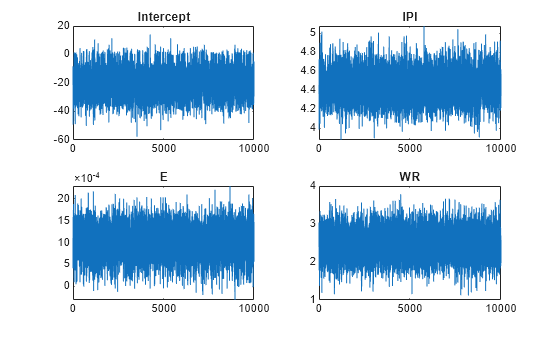
figure;
plot(PosteriorMdl.Sigma2Draws);
title('Sigma2');
The trace plots indicate that the draws seem to mix well. The plots show no detectable transience or serial correlation, and the draws do not jump between states.
Consider the linear regression model in Create Prior Model for SSVS.
Load the Nelson-Plosser data set. Create variables for the response and predictor series.
load Data_NelsonPlosser
VarNames = ["IPI" "E" "WR"];
X = DataTable{:,VarNames};
y = DataTable{:,"GNPR"};
Assume the following:
The intercept is in the model with probability 0.9.
IPIandEare in the model with probability 0.75.If
Eis included in the model, then the probability thatWRis included in the model is 0.9.If
Eis excluded from the model, then the probability thatWRis included is 0.25.
Declare a function named priorssvsexample.m that:
Accepts a logical vector indicating whether the intercept and variables are in the model (
truefor model inclusion). Element 1 corresponds to the intercept, and the rest of the elements correspond to the variables in the data.Returns a numeric scalar representing the log of the described prior regime probability distribution.
function logprior = priorssvsexample(varinc)
%PRIORSSVSEXAMPLE Log prior regime probability distribution for SSVS
%   PRIORSSVSEXAMPLE is an example of a custom log prior regime probability
%   distribution for SSVS with dependent random variables. varinc is
%   a 4-by-1 logical vector indicating whether 4 coefficients are in a model
%   and logPrior is a numeric scalar representing the log of the prior
%   distribution of the regime probabilities.
%
%   Coefficients enter a model according to these rules:
%       * varinc(1) is included with probability 0.9.
%       * varinc(2) and varinc(3) are in the model with probability 0.75.
%       * If varinc(3) is included in the model, then the probability that
%       varinc(4) is included in the model is 0.9.
%       * If varinc(3) is excluded from the model, then the probability
%       that varinc(4) is included is 0.25.

logprior = log(0.9) + 2*log(0.75) + log(varinc(3)*0.9 + (1-varinc(3))*0.25);

end
Create a prior model for performing SSVS. Assume that  and
and  are (a conjugate mixture model). Specify the number of predictors
 p the names of the regression coefficients, and custom, prior probability distribution of the variable-inclusion regimes.
p = 3;
PriorMdl = mixconjugateblm(p,'VarNames',["IPI" "E" "WR"],...
    'Probability',@priorssvsexample);
Implement SSVS by estimating the marginal posterior distributions of and . Because SSVS uses MCMC for estimation, set a random number seed to reproduce the results.
rng(1);
PosteriorMdl = estimate(PriorMdl,X,y);
Method: MCMC sampling with 10000 draws
Number of observations: 62
Number of predictors:   4

           |   Mean      Std           CI95        Positive  Distribution  Regime
----------------------------------------------------------------------------------
 Intercept | -18.7971  10.1644  [-37.002,  0.765]    0.039     Empirical   0.8797
 IPI       |   4.4559   0.1530   [ 4.166,  4.760]    1.000     Empirical   0.4623
 E         |   0.0010   0.0004   [ 0.000,  0.002]    0.997     Empirical   0.2665
 WR        |   2.4684   0.3618   [ 1.759,  3.196]    1.000     Empirical   0.1727
 Sigma2    |  47.7391   8.6741   [33.823, 67.024]    1.000     Empirical    NaN
Assuming, that variables with Regime < 0.1 should be removed from the model, the results suggest that you can include all variables in the model.
Consider the regression model in Create Prior Model for SSVS.
Perform SSVS:
Create a Bayesian regression model for SSVS with a conjugate prior for the data likelihood. Use the default settings.
Hold out the last 10 periods of data from estimation.
Estimate the marginal posterior distributions.
p = 3;
PriorMdl = bayeslm(p,'ModelType','mixconjugate','VarNames',["IPI" "E" "WR"]);

load Data_NelsonPlosser
fhs = 10; % Forecast horizon size
X = DataTable{1:(end - fhs),PriorMdl.VarNames(2:end)};
y = DataTable{1:(end - fhs),'GNPR'};
XF = DataTable{(end - fhs + 1):end,PriorMdl.VarNames(2:end)}; % Future predictor data
yFT = DataTable{(end - fhs + 1):end,'GNPR'};                  % True future responses

rng(1); % For reproducibility
PosteriorMdl = estimate(PriorMdl,X,y,'Display',false);
Forecast responses using the posterior predictive distribution and the future predictor data XF. Plot the true values of the response and the forecasted values.
yF = forecast(PosteriorMdl,XF);

figure;
plot(dates,DataTable.GNPR);
hold on
plot(dates((end - fhs + 1):end),yF)
h = gca;
hp = patch([dates(end - fhs + 1) dates(end) dates(end) dates(end - fhs + 1)],...
    h.YLim([1,1,2,2]),[0.8 0.8 0.8]);
uistack(hp,'bottom');
legend('Forecast Horizon','True GNPR','Forecasted GNPR','Location','NW')
title('Real Gross National Product: 1909 - 1970');
ylabel('rGNP');
xlabel('Year');
hold off
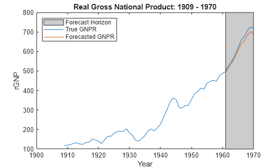
yF is a 10-by-1 vector of future values of real GNP corresponding to the future predictor data.
Estimate the forecast root mean squared error (RMSE).
frmse = sqrt(mean((yF - yFT).^2))
frmse =
18.8470
The forecast RMSE is a relative measure of forecast accuracy. Specifically, you estimate several models using different assumptions. The model with the lowest forecast RMSE is the best-performing model of the ones being compared.
When you perform Bayesian regression with SSVS, a best practice is to tune the hyperparameters. One way to do so is to estimate the forecast RMSE over a grid of hyperparameter values, and choose the value that minimizes the forecast RMSE.
More About
Algorithms
A closed-form posterior exists for conjugate mixture priors in the SSVS framework with K coefficients. However, because the prior β|σ2,γ, marginalized by γ, is a 2K-component Gaussian mixture, MATLAB® uses MCMC instead to sample from the posterior for numerical stability.
Alternative Functionality
The bayeslm function can create any supported prior model object for Bayesian linear regression.
References
[1] George, E. I., and R. E. McCulloch. "Variable Selection Via Gibbs Sampling." Journal of the American Statistical Association. Vol. 88, No. 423, 1993, pp. 881–889.
[2] Koop, G., D. J. Poirier, and J. L. Tobias. Bayesian Econometric Methods. New York, NY: Cambridge University Press, 2007.
Version History
Introduced in R2018b