Convergence of AR Forecasts
This example shows how to forecast a stationary AR(12) process using forecast. Evaluate the asymptotic convergence of the forecasts, and compare forecasts made with and without using presample data.
Step 1. Specify an AR(12) model.
Specify the model
where the innovations are Gaussian with variance 2. Generate a realization of length 300 from the process. Discard the first 250 observations as burn-in.
Mdl = arima('Constant',3,'AR',{0.7,0.25},'ARLags',[1,12],...
              'Variance',2);

rng('default')
Y = simulate(Mdl,300);
Y = Y(251:300);

figure
plot(Y)
xlim([0,50])
title('Simulated AR(12) Process')

Step 2. Forecast the process using presample data.
Generate forecasts (and forecast errors) for a 150-step time horizon. Use the simulated series as presample data.
[Yf,YMSE] = forecast(Mdl,150,Y);
upper = Yf + 1.96*sqrt(YMSE);
lower = Yf - 1.96*sqrt(YMSE);

figure
plot(Y,'Color',[.75,.75,.75])
hold on
plot(51:200,Yf,'r','LineWidth',2)
plot(51:200,[upper,lower],'k--','LineWidth',1.5)
xlim([0,200])
hold off

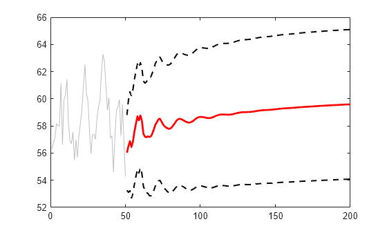
The MMSE forecast sinusoidally decays, and begins converging to the unconditional mean, given by
Step 3. Calculate the asymptotic variance.
The MSE of the process converges to the unconditional variance of the process (). You can calculate the variance using the impulse response function. The impulse response function is based on the infinite-degree MA representation of the AR(2) process.
The last few values of YMSE show the convergence toward the unconditional variance.
ARpol = LagOp({1,-.7,-.25},'Lags',[0,1,12]);
IRF = cell2mat(toCellArray(1/ARpol));
sig2e = 2;

variance = sum(IRF.^2)*sig2e % Display the variance
variance = 7.9938
YMSE(145:end) % Display the forecast MSEsans = 6×1
7.8870
7.8899
7.8926
7.8954
7.8980
7.9006
Convergence is not reached within 150 steps, but the forecast MSE is approaching the theoretical unconditional variance.
Step 4. Forecast without using presample data.
Repeat the forecasting without using any presample data.
[Yf2,YMSE2] = forecast(Mdl,150);
upper2 = Yf2 + 1.96*sqrt(YMSE2);
lower2 = Yf2 - 1.96*sqrt(YMSE2);

YMSE2(145:end) % Display the forecast MSEs
ans = 6×1
7.8870
7.8899
7.8926
7.8954
7.8980
7.9006
figure
plot(Y,'Color',[.75,.75,.75])
hold on
plot(51:200,Yf2,'r','LineWidth',2)
plot(51:200,[upper2,lower2],'k--','LineWidth',1.5)
xlim([0,200])
hold off

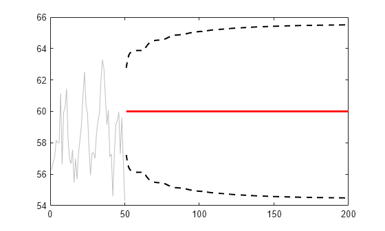
The convergence of the forecast MSE is the same without using presample data. However, all MMSE forecasts are the unconditional mean. This is because forecast initializes the AR model with the unconditional mean when you do not provide presample data.