designRateConverter
Description
filtObj = designRateConverter(Name=Value)
For example, filtObj =
designRateConverter(InterpolationFactor=36,DecimationFactor=2,MaxStages=3,Bandwidth=1/72)
designs a 36:2 or 18:1 rate converter with a maximum of three stages, and an input bandwidth
of 1/72 in normalized frequency units. In normalized units, the input Nyquist frequency is
1, so the bandwidth in this case is 1/72 of that Nyquist frequency. Given these argument
values, the function returns a three-stage cascade of dsp.FIRInterpolator System objects with an interpolation factor of 3, 2, and 3,
respectively, for the three stages.
The designRateConverter function outputs the design configuration
(number of stages and specifications of each stage) that has the least number of
multiplications per input sample (MPIS). By default, the function estimates this cost and
designs the default configuration based on this value. You can
choose to minimize the total number of filter coefficients instead using the
OptimizeFor property (since R2025a).
When you specify only a partial list of filter parameters, the function designs the
filter by setting the other design parameters to their default values. When you set
Verbose = true, the function returns the values of
all the design parameters and the effective conversion ratio.
Examples
Design a multistage decimator with these specifications using the designRateConverter function:
Decimation factor of 36
Input bandwidth of interest set to 0.01 in normalized frequency units
Design two filters with MaxStages set to 2 and Inf, respectively. Setting MaxStages to 2 means that the design must have a maximum of two stages. Setting MaxStages to Inf allows the function to use as many stages as needed to obtain an optimal design. Compare the cost of implementing the two filters.
Use the designRateConverter to design the multistage decimator. Set DecimationFactor to 36, Bandwidth to 0.01, and MaxStages to 2. Setting Verbose to true displays the values of the other arguments the function uses. When you specify only a partial list of function arguments, the function sets the other design parameters to their default values.
decimTwoStages = designRateConverter(DecimationFactor=36,...
    Bandwidth=0.01,MaxStages=2,Verbose=true)
designRateConverter(InterpolationFactor=1, DecimationFactor=36, Bandwidth=0.01, StopbandAttenuation=80, MaxStages=2, CostMethod="estimate", OptimizeFor="MPIS", Tolerance=0, ToleranceUnits="absolute") Conversion ratio: 1:36
decimTwoStages =
  dsp.FilterCascade with properties:

         Stage1: [1×1 dsp.FIRDecimator]
         Stage2: [1×1 dsp.FIRDecimator]
    CloneStages: true
Design another filter by setting MaxStages to Inf. This setting allows the function to choose the optimal number of stages for designing the filter. The function designs the filter as a decimator cascade of three stages with decimation factors equal to 2, 3, and 3, respectively, for the three stages.
decimMaxStages = designRateConverter(DecimationFactor=36,MaxStages=Inf,...
    Bandwidth=0.01,Verbose=true)
designRateConverter(InterpolationFactor=1, DecimationFactor=36, Bandwidth=0.01, StopbandAttenuation=80, MaxStages=Inf, CostMethod="estimate", OptimizeFor="MPIS", Tolerance=0, ToleranceUnits="absolute") Conversion ratio: 1:36
decimMaxStages =
  dsp.FilterCascade with properties:

         Stage1: [1×1 dsp.FIRDecimator]
         Stage2: [1×1 dsp.FIRDecimator]
         Stage3: [1×1 dsp.FIRDecimator]
    CloneStages: true
View the filter information using the info function.
info(decimMaxStages)
ans =
    'Discrete-Time Filter Cascade
     ----------------------------
     Number of stages: 3
     Stage cloning: enabled
     Input sample rate: Normalized
     ----------------------------

     Stage1: dsp.FIRDecimator
     -------
     Discrete-Time FIR Multirate Filter (real)
     -----------------------------------------
     Filter Structure   : Direct-Form FIR Polyphase Decimator
     Decimation Factor  : 2
     Polyphase Length   : 4
     Filter Length      : 7
     Stable             : Yes
     Linear Phase       : Yes (Type 1)

     Arithmetic         : double
     Input sample rate : 1


     Stage2: dsp.FIRDecimator
     -------
     Discrete-Time FIR Multirate Filter (real)
     -----------------------------------------
     Filter Structure   : Direct-Form FIR Polyphase Decimator
     Decimation Factor  : 2
     Polyphase Length   : 6
     Filter Length      : 11
     Stable             : Yes
     Linear Phase       : Yes (Type 1)

     Arithmetic         : double
     Input sample rate : 0.5


     Stage3: dsp.FIRDecimator
     -------
     Discrete-Time FIR Multirate Filter (real)
     -----------------------------------------
     Filter Structure   : Direct-Form FIR Polyphase Decimator
     Decimation Factor  : 9
     Polyphase Length   : 8
     Filter Length      : 67
     Stable             : Yes
     Linear Phase       : Yes (Type 1)

     Arithmetic         : double
     Input sample rate : 0.25

     '
Compare Cost
Compare the cost of implementing the two filters. The cost on all metrics reduces when you remove the restriction on the maximum number of stages.
cost(decimTwoStages)
ans = struct with fields:
                  NumCoefficients: 130
                        NumStates: 132
    MultiplicationsPerInputSample: 5.9722
          AdditionsPerInputSample: 5.4444
cost(decimMaxStages)
ans = struct with fields:
                  NumCoefficients: 73
                        NumStates: 79
    MultiplicationsPerInputSample: 5.9444
          AdditionsPerInputSample: 5.1667
Compare Magnitude Response
Compare the magnitude response of the two filters. Both filters display similar behavior in the transition band.
filterAnalyzer(decimTwoStages,decimMaxStages,FilterNames=["TwoStages","ThreeStages"])
However, to understand the source of computational savings in the three-stage design, analyze the magnitude response of the three stages individually.
stage1 = decimMaxStages.Stage1
stage1 =
  dsp.FIRDecimator with properties:

   Main
    DecimationFactor: 2
     NumeratorSource: 'Property'
           Numerator: [-0.0317 0 0.2817 0.5000 0.2817 0 -0.0317]
           Structure: 'Direct form'

  Show all properties
stage2 = decimMaxStages.Stage2
stage2 =
  dsp.FIRDecimator with properties:

   Main
    DecimationFactor: 2
     NumeratorSource: 'Property'
           Numerator: [0.0065 0 -0.0507 0 0.2942 0.5000 0.2942 0 -0.0507 0 0.0065]
           Structure: 'Direct form'

  Show all properties
stage3 = decimMaxStages.Stage3
stage3 =
  dsp.FIRDecimator with properties:

   Main
    DecimationFactor: 9
     NumeratorSource: 'Property'
           Numerator: [-9.6325e-05 -1.5539e-04 -2.4072e-04 -3.0942e-04 -3.2259e-04 -2.3401e-04 0 4.0676e-04 9.8161e-04 0.0017 0.0024 0.0029 0.0032 0.0029 0.0018 0 -0.0026 -0.0058 -0.0092 -0.0123 -0.0145 -0.0149 -0.0129 -0.0081 0 0.0113 … ] (1×67 double)
           Structure: 'Direct form'

  Show all properties
The third stage provides the narrow transition width required for the overall design. However, the third stage contains spectral replicas. The first stage removes such replicas. The first and second stages operate at a faster rate but can afford a wider transition width. The result is a decimate-by-2 first-stage filter with only five nonzero coefficients and decimate-by-2 second-stage filter with only seven nonzero coefficients. The third stage contains 61 nonzero coefficients. Overall, the three-stage design uses 73 nonzero coefficients, while the two-stage design uses 130 nonzero coefficients.
filterAnalyzer(stage1,stage2,stage3,FilterNames=["Stage1","Stage2","Stage3"])

Since R2025a
Design two multistage decimators with the same design specifications but different cost minimization objectives.
Filter Design
Here are the filter design specifications:
Decimation factor of 48
Input bandwidth of interest of 0.019 in normalized frequency units
M  = 48;
BW = 0.019;
Use the designRateConverter function to design the filters. Set the OptimizeFor property to Total Coefficients and MPIS, respectively. The designRateConverter function minimizes the total number of filter coefficients in the first filter and the number of multiplications per input sample in the second filter.
minCoeffDecim_TC = designRateConverter(DecimationFactor=M,...
    Bandwidth=BW,OptimizeFor="Total Coefficients")
minCoeffDecim_TC =
  dsp.FilterCascade with properties:

         Stage1: [1×1 dsp.FIRDecimator]
         Stage2: [1×1 dsp.FIRDecimator]
         Stage3: [1×1 dsp.FIRDecimator]
         Stage4: [1×1 dsp.FIRDecimator]
         Stage5: [1×1 dsp.FIRDecimator]
    CloneStages: true
minCoeffDecim_MPIS = designRateConverter(DecimationFactor=M,...
    Bandwidth=BW,OptimizeFor="MPIS")
minCoeffDecim_MPIS =
  dsp.FilterCascade with properties:

         Stage1: [1×1 dsp.FIRDecimator]
         Stage2: [1×1 dsp.FIRDecimator]
         Stage3: [1×1 dsp.FIRDecimator]
         Stage4: [1×1 dsp.FIRDecimator]
         Stage5: [1×1 dsp.FIRDecimator]
    CloneStages: true
Compare Cost
Compare the cost of implementing the two filters. Even with the same design specifications, the first filter has fewer filter coefficients while the second filter has fewer multiplications per input sample.
cost(minCoeffDecim_TC)
ans = struct with fields:
                  NumCoefficients: 91
                        NumStates: 155
    MultiplicationsPerInputSample: 6.8542
          AdditionsPerInputSample: 6.0417
cost(minCoeffDecim_MPIS)
ans = struct with fields:
                  NumCoefficients: 95
                        NumStates: 158
    MultiplicationsPerInputSample: 6.7292
          AdditionsPerInputSample: 5.7917
Design a multistage interpolator with these specifications using the designRateConverter function:
Interpolation factor of 23
Input bandwidth of interest set to 0.1 in normalized frequency units
Design two filters with CostMethod set to "estimate" and "design", respectively. Compare the cost of the two designs.
Use designRateConverter to design the multistage interpolator. Set InterpolationFactor to 128 and Bandwidth to 0.1. Set Verbose to true to display the default values of the other arguments. When you specify only a partial list of function arguments, the function sets the other design parameters to their default values. The function sets CostMethod to "estimate" by default. The function determines the design configuration (number of stages and specifications for each stage) based on the estimated cost.
interpEstimateCost = designRateConverter(InterpolationFactor=128,...
    Bandwidth=0.1,Verbose=true)
designRateConverter(InterpolationFactor=128, DecimationFactor=1, Bandwidth=0.1, StopbandAttenuation=80, MaxStages=Inf, CostMethod="estimate", OptimizeFor="MPIS", Tolerance=0, ToleranceUnits="absolute") Conversion ratio: 128:1
interpEstimateCost =
  dsp.FilterCascade with properties:

         Stage1: [1×1 dsp.FIRInterpolator]
         Stage2: [1×1 dsp.FIRInterpolator]
         Stage3: [1×1 dsp.FIRInterpolator]
    CloneStages: true
Change CostMethod to "design". The function optimizes the design with respect to the exact cost rather than the estimated cost. Notice that the design now uses four stages.
interpDesignCost = designRateConverter(InterpolationFactor=128,...
    Bandwidth=0.1,CostMethod="design",Verbose=true)
designRateConverter(InterpolationFactor=128, DecimationFactor=1, Bandwidth=0.1, StopbandAttenuation=80, MaxStages=Inf, CostMethod="design", OptimizeFor="MPIS", Tolerance=0, ToleranceUnits="absolute")

Conversion ratio: 128:1
interpDesignCost =
  dsp.FilterCascade with properties:

         Stage1: [1×1 dsp.FIRInterpolator]
         Stage2: [1×1 dsp.FIRInterpolator]
         Stage3: [1×1 dsp.FIRInterpolator]
         Stage4: [1×1 dsp.FIRInterpolator]
    CloneStages: true
Compare Cost
Compute the cost of implementing the two filters. When you set CostMethod to "estimate", the function finds a suboptimal solution. Setting CostMethod to "design" allows the function to obtain an optimal solution, at the expense of the runtime performance of the design algorithm.
cost(interpEstimateCost)
ans = struct with fields:
                  NumCoefficients: 170
                        NumStates: 11
    MultiplicationsPerInputSample: 546
          AdditionsPerInputSample: 419
cost(interpDesignCost)
ans = struct with fields:
                  NumCoefficients: 92
                        NumStates: 14
    MultiplicationsPerInputSample: 528
          AdditionsPerInputSample: 401
Compare Magnitude Response
Compare the magnitude response. Both filters display similar behavior in the transition band but behave differently in the stopband.
filterAnalyzer(interpEstimateCost,interpDesignCost,FilterNames=["Estimate","Design"])

Design a multistage sample-rate converter with these specifications using the designRateConverter function:
Input sample rate of 48 kHz
Output sample rate of 44.1 kHz
Design two filters with the output tolerance of 0 Hz and 220 Hz, respectively. Changing the output tolerance allows the output sample rate to vary by up to 220 Hz from the specified value of 44.1 kHz. Compare the cost of implementing the two filters.
Use the designRateConverter to design the multistage sample-rate converter. Set InputSampleRate to 48 kHz, OutputSampleRate to 44.1 kHz, and Tolerance to 0. Set Verbose to true to display the values of the other arguments. When you specify only a partial list of function arguments, the function sets the other design parameters to their default values.
The function uses an effective conversion ratio of 147:160, which is high.
designExactRate = designRateConverter(InputSampleRate=48e3,OutputSampleRate=44.1e3,...
    Tolerance=0,Verbose=true)
designRateConverter(InputSampleRate=48000, OutputSampleRate=44100, Bandwidth=17640, StopbandAttenuation=80, MaxStages=Inf, CostMethod="estimate", OptimizeFor="MPIS", Tolerance=0, ToleranceUnits="absolute") Conversion ratio: 147:160 Input sample rate: 48000 Output sample rate: 44100
designExactRate =
  dsp.FIRRateConverter with properties:

   Main
    InterpolationFactor: 147
       DecimationFactor: 160
        NumeratorSource: 'Property'
              Numerator: [6.1512e-05 6.2675e-05 6.3826e-05 6.4965e-05 6.6092e-05 6.7203e-05 6.8300e-05 6.9379e-05 7.0441e-05 7.1484e-05 7.2507e-05 7.3508e-05 7.4487e-05 7.5442e-05 7.6372e-05 7.7276e-05 7.8153e-05 7.9001e-05 7.9819e-05 … ] (1×4017 double)

  Show all properties
Allow a tolerance of 220 Hz. The function now uses a conversion ratio of 11:12 which has less computational complexity.
designApproximateRate = designRateConverter(InputSampleRate=48e3,OutputSampleRate=44.1e3,...
    Tolerance=220,Verbose=true)
designRateConverter(InputSampleRate=48000, OutputSampleRate=44100, Bandwidth=17600, StopbandAttenuation=80, MaxStages=Inf, CostMethod="estimate", OptimizeFor="MPIS", Tolerance=220, ToleranceUnits="absolute") Conversion ratio: 11:12 Input sample rate: 48000 Output sample rate: 44100 (specified) 44000 (effective)
designApproximateRate =
  dsp.FIRRateConverter with properties:

   Main
    InterpolationFactor: 11
       DecimationFactor: 12
        NumeratorSource: 'Property'
              Numerator: [3.8374e-05 5.7656e-05 7.7489e-05 9.5302e-05 1.0809e-04 1.1269e-04 1.0611e-04 8.5908e-05 5.0600e-05 0 -6.4471e-05 -1.3962e-04 -2.2046e-04 -3.0037e-04 -3.7143e-04 -4.2502e-04 -4.5247e-04 -4.4592e-04 -3.9922e-04 … ] (1×307 double)

  Show all properties
Compare Cost
Compute the cost of implementing the two filters. Allowing some tolerance in the output sample rate reduces the cost of the filter.
cost(designExactRate)
ans = struct with fields:
                  NumCoefficients: 3993
                        NumStates: 27
    MultiplicationsPerInputSample: 24.9563
          AdditionsPerInputSample: 24.0375
cost(designApproximateRate)
ans = struct with fields:
                  NumCoefficients: 283
                        NumStates: 27
    MultiplicationsPerInputSample: 23.5833
          AdditionsPerInputSample: 22.6667
Compare Magnitude Response and Group Delay
Compare the magnitude response of the two filters. The filter with zero tolerance has a very narrow transition width, while allowing some tolerance increases the transition width and the passband width.
filterAnalyzer(designExactRate,designApproximateRate,FilterNames=["ZeroTolerance","HigherTolerance"])

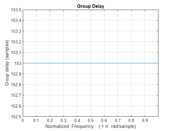
Compare the group delay of the two filters. The filter with zero tolerance has a group delay of 2008 samples, while the allowing some tolerance decreases the group delay significantly to 153.
grpdelay(designExactRate)
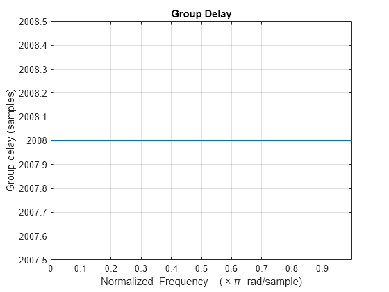
grpdelay(designApproximateRate)
Design a multistage sample-rate converter with these specifications using the designRateConverter function:
Interpolation factor of 3756
Decimation factor of 6200
Design three filters with the tolerance percentage of 0%, 0.1%, and 1%. Compare the cost of implementing these filters.
Use the designRateConverter to design the multistage sample-rate converter. Set InterpolationFactor to 3756, DecimationFactor to 6200, and ToleranceUnits to "percentage". The default value of Tolerance is 0. Set Verbose to true to display the default values of the other arguments. When you specify only a partial list of function arguments, the function sets the other design parameters to their default values.
The function uses an effective conversion ratio of 939:1550 since it removes the common denominator 4 from the specified conversion ratio of 3756:6200.
designExactRate = designRateConverter(InterpolationFactor=3756,...
    DecimationFactor=6200,ToleranceUnits="percentage",...
    Verbose=true)
designRateConverter(InterpolationFactor=3756, DecimationFactor=6200, Bandwidth=0.48464516129032265, StopbandAttenuation=80, MaxStages=Inf, CostMethod="estimate", OptimizeFor="MPIS", Tolerance=0, ToleranceUnits="percentage")

Conversion ratio: 3756:6200 (specified), 939:1550 (effective)
designExactRate =
  dsp.FIRRateConverter with properties:

   Main
    InterpolationFactor: 939
       DecimationFactor: 1550
        NumeratorSource: 'Property'
              Numerator: [4.0641e-05 4.0719e-05 4.0798e-05 4.0876e-05 4.0955e-05 4.1033e-05 4.1111e-05 4.1190e-05 4.1268e-05 4.1346e-05 4.1424e-05 4.1502e-05 4.1580e-05 4.1657e-05 4.1735e-05 4.1813e-05 4.1890e-05 4.1967e-05 … ] (1×38895 double)

  Show all properties
Set Tolerance to 0.1%. The effective conversion ratio changes to 20:33, which is very close to the specified ratio of 3756/6200. 3756/6200-20/33 = 2.5415e-04, which is within the allowed tolerance of 1e-3 (or 0.1%).
designApproxRate = designRateConverter(InterpolationFactor=3756,...
    DecimationFactor=6200,ToleranceUnits="percentage",...
    Tolerance=0.1,Verbose=true)
designRateConverter(InterpolationFactor=3756, DecimationFactor=6200, Bandwidth=0.48484848484848486, StopbandAttenuation=80, MaxStages=Inf, CostMethod="estimate", OptimizeFor="MPIS", Tolerance=0.1, ToleranceUnits="percentage")

Conversion ratio: 3756:6200 (specified), 20:33 (effective)
designApproxRate =
  dsp.FIRRateConverter with properties:

   Main
    InterpolationFactor: 20
       DecimationFactor: 33
        NumeratorSource: 'Property'
              Numerator: [2.7533e-05 3.2037e-05 3.6669e-05 4.1362e-05 4.6039e-05 5.0621e-05 5.5019e-05 5.9141e-05 6.2891e-05 6.6170e-05 6.8878e-05 7.0914e-05 7.2179e-05 7.2576e-05 7.2015e-05 7.0409e-05 6.7680e-05 6.3762e-05 5.8596e-05 … ] (1×841 double)

  Show all properties
Increase the tolerance to 1%. The effective conversion ratio further reduces to 3:5. 3756/6200-3/5 = 0.0058, which is within the allowed tolerance of 0.01 (or 1%).
designApproxRateHigherTol = designRateConverter(InterpolationFactor=3756,...
    DecimationFactor=6200,ToleranceUnits="percentage",...
    Tolerance=1,Verbose=true)
designRateConverter(InterpolationFactor=3756, DecimationFactor=6200, Bandwidth=0.48, StopbandAttenuation=80, MaxStages=Inf, CostMethod="estimate", OptimizeFor="MPIS", Tolerance=1, ToleranceUnits="percentage")

Conversion ratio: 3756:6200 (specified), 3:5 (effective)
designApproxRateHigherTol =
  dsp.FIRRateConverter with properties:

   Main
    InterpolationFactor: 3
       DecimationFactor: 5
        NumeratorSource: 'Property'
              Numerator: [2.0191e-05 5.1900e-05 7.6263e-05 6.5863e-05 0 -1.1657e-04 -2.4237e-04 -3.0607e-04 -2.3543e-04 0 3.5191e-04 6.8589e-04 8.1926e-04 6.0023e-04 0 -8.2688e-04 -0.0016 -0.0018 -0.0013 0 0.0017 0.0031 0.0035 0.0024 0 … ] (1×129 double)

  Show all properties
Compare Cost
Compute the cost of implementing these filters. As you increase the tolerance, the computational complexity of the filter reduces.
cost(designExactRate)
ans = struct with fields:
                  NumCoefficients: 38871
                        NumStates: 41
    MultiplicationsPerInputSample: 25.0781
          AdditionsPerInputSample: 24.4723
cost(designApproxRate)
ans = struct with fields:
                  NumCoefficients: 817
                        NumStates: 42
    MultiplicationsPerInputSample: 24.7576
          AdditionsPerInputSample: 24.1515
cost(designApproxRateHigherTol)
ans = struct with fields:
                  NumCoefficients: 105
                        NumStates: 42
    MultiplicationsPerInputSample: 21
          AdditionsPerInputSample: 20.4000
Compare Magnitude Response and Group Delay
Compare the magnitude response of the filters. The filter with zero tolerance has the least transition width and the transition width increases as the tolerance increases.
filterAnalyzer(designExactRate,designApproxRate,designApproxRateHigherTol,...
    FilterNames=["ZeroTolerance","OneTenthPercentTolerance","OnePercentTolerance"])
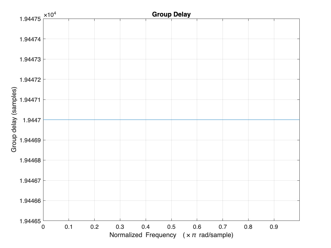
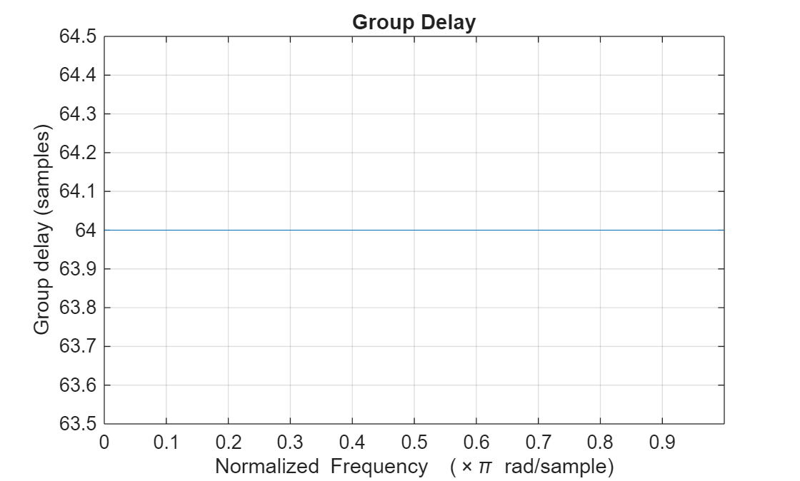
Comparing the group delay values, you can see that the filter with zero tolerance has a significantly higher group delay of 19447.1 samples. As tolerance increases, the group delay reduces. For a tolerance of 1%, the group delay reduces to 64 samples.
grpdelay(designExactRate)
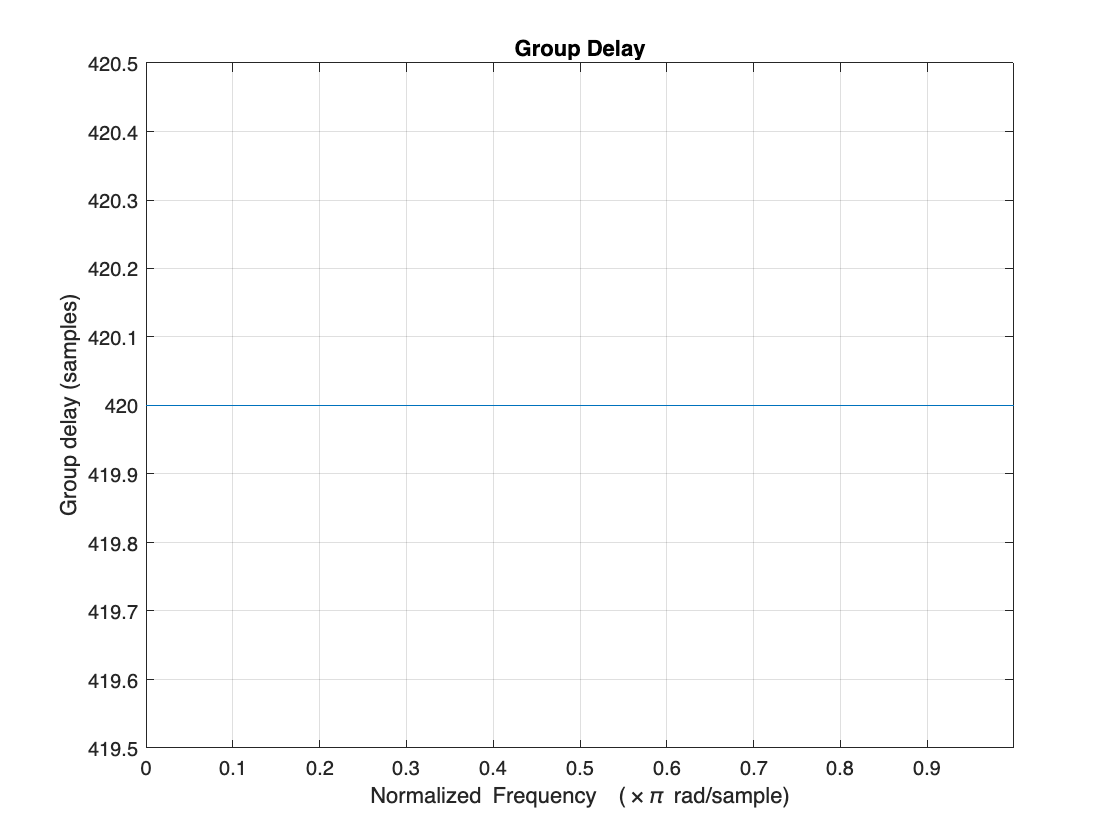
grpdelay(designApproxRate)
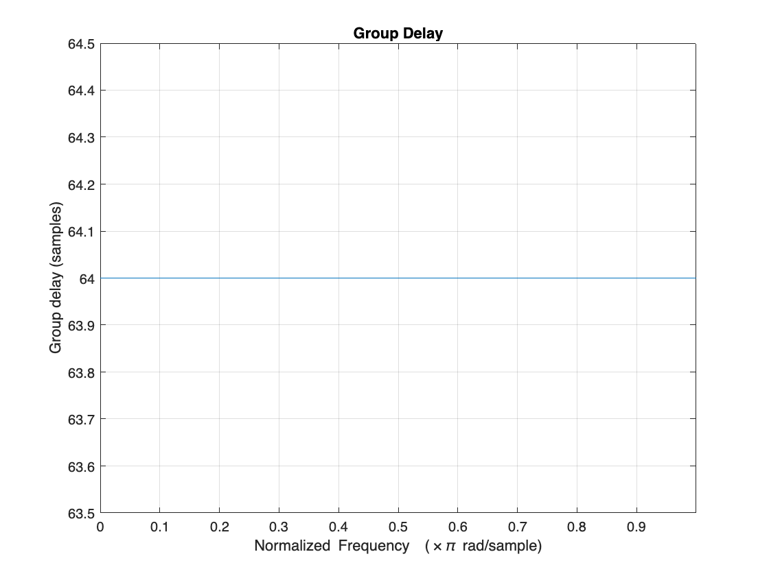
grpdelay(designApproxRateHigherTol)
Name-Value Arguments
Output Arguments
Algorithms
The function splits the overall interpolation and decimation factors into smaller factors, with each factor corresponding to the individual stage. The combined rate conversion factor of all the individual stages must equal the overall rate conversion factor. The combined response must meet or exceed the given design specifications.
The function determines the number of stages and the sequence of stages based on the
overall implementation cost. The function chooses the configuration that has the least
implementation cost. Depending on the setting of CostMethod, the function
estimates the cost or determines it exactly for a specific design configuration. The
estimation method is faster but can lead to suboptimal designs. The design method takes longer
but gives an accurate overall cost of implementation.
You can further specify which type of cost metric to
minimize, multiplications per input sample (MPIS), or the total number of filter coefficients,
by setting the OptimizeFor property appropriately. In many cases, the
optimal filter design minimizes both the MPIS and the number of coefficients. However, there
are filter configurations where the function optimizes one over the other. For an example, see
Design Multistage Decimator with Different Cost Minimizations. (since R2025a)