Verify Global Stability of ACAS Xu Neural Networks

Since R2026a

This example uses:

This example shows how to verify global robustness and stability of an ACAS Xu neural network across the entire operational design domain (ODD). This example is step 3 in a series of examples that take you through formally verifying a set of neural networks that output steering advisories to aircraft to prevent them from colliding with other aircraft.

To run this example, open Verify and Deploy Airborne Collision Avoidance System (ACAS) Xu Neural Networks and navigate to Step3VerifyGlobalStabilityOfACASXuNeuralNetworkExample.m. This project contains all of the steps for this workflow. You can run the scripts in order or run each one independently.

By default, the example uses one or more GPUs if they are available. Using a GPU requires a Parallel Computing Toolbox™ license and a supported GPU device. For information on supported devices, see GPU Computing Requirements (Parallel Computing Toolbox). Otherwise, the example uses the CPU.

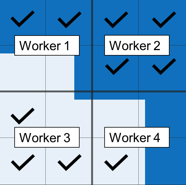
The example splits the ODD into equal hypercuboid sections and verifies local stability on each section. For greater speed, this example automatically runs in parallel if you have Parallel Computing Toolbox™ installed.

Diagram illustrating the ODD split into equal hypercuboid sections, with a decision boundary running through the middle.

Stability and Robustness

Stability and robustness are both measures of how susceptible a neural network is to input perturbations. A network is stable if the network output does not change drastically due to small changes to the network input. A network is robust if it is both stable and correct. A neural network can be locally stable or robust within a subsection of the ODD, or it can be globally stable or robust across the entire ODD.

Depending on your workflow, you may have a requirement about the maximum change of network output $δ$ given a maximum change in network input $ϵ$ , or vice versa. Formal methods allow you to prove or disprove that your network fulfills these requirements. There are four different properties that you can prove:

Local Stability — A neural network is locally stable within a region centered around a point $x_{0}$ within the ODD when inputs that are close to each other yield outputs that are close to each other.

$| x - x_{0} |_{p} \leq ϵ \to | f (x) - f (x_{0}) |_{p} \leq δ$

Global Stability — A neural network is globally stable across the entire ODD if the network is locally stable at every element of the ODD.

$\forall x_{i}, x_{j}, \in D | x_{i} - x_{j} |_{p} \leq ϵ \to | f (x_{i}) - f (x_{j}) |_{p} \leq δ$

Local Robustness — A neural network is locally robust within a region centered around a point $x_{0}$ within the ODD when inputs that are close to $x_{0}$ result in outputs that are close to the true answer at $x_{0}$ .

$| x - x_{0} |_{p} \leq ϵ \to | f (x) - y_{true} (x_{0}) |_{p} \leq δ$

Global Robustness — A neural network is globally robust across the entire ODD if the network is locally robust at every element of the ODD.

$\forall x_{i}, x_{j}, \in D | x_{i} - x_{j} |_{p} \leq ϵ \to | f (x_{i}) - y_{true} (x_{j}) |_{p} \leq δ$

Here, $D$ is the operational design domain, $f$ is the neural network function, $y_{true}$ is the ground truth, and $| . . . |_{p}$ denotes the choice of norm. To split up the ODD into local regions with no overlap or gaps, this example uses the $p = \infty$ norm. The set of $x$ such that $| x - x_{0} |_{\infty} \leq ϵ$ is a hypercube.

To define an asymmetric region, such as a rectangle rather than a square, you can include a scaling factor to rescale the dimensions. That is, apply $| (x - x_{0}) / ω |_{\infty} \leq ϵ$ , where $ω$ applies a scale factor in each dimension.

For convenience, you can define the input region in terms of its upper and lower bounds, $x_{l}, x_{u}$ , instead of its center $x_{0}$ and distance to the edges $ϵ$ . For example, the estimateNetworkOutputBounds function uses $x_{l}, x_{u}$ to define the input region.

For classification networks, the network output is a discrete classification label. It is not always useful to apply the above definitions to the discrete labels. A classification network with decision boundaries is not necessarily vulnerable to adversarial examples. Instead, you can apply the stability and robustness definitions to the network output scores associated with the different classes.

Load ACAS Xu Neural Networks

Load and save the networks. The example prepares the networks as shown in Explore ACAS Xu Neural Networks.

acasXuNetworkFolder = fullfile(matlab.project.rootProject().RootFolder,".");
zipFile = matlab.internal.examples.downloadSupportFile("nnet","data/acas-xu-neural-network-dataset.zip");
filepath = fileparts(zipFile);
unzip(zipFile,acasXuNetworkFolder);
matFolder = fullfile(matlab.project.rootProject().RootFolder,"acas-xu-neural-network-dataset","networks-mat");
helpers.convertACASXuFromONNXAndSave(matFolder);

Importing ONNX files and converting to MAT format...
.........    ..........    ..........    ..........    ......
Import and conversion complete.

Explore Local Stability Across ODD

In this section, to verify the global stability and robustness across the entire operational design domain (ODD), split the ODD into smaller sections and verify local stability and robustness within the smaller sections.

Define ODD

The ODD is the space of all valid inputs to a network.

For the ACAS Xu family of neural networks, the network input consists of five scalars, each bounded from both above and below.

Network Input	Description	Units	Range/Values [3][4]
$ρ$	Distance from ownship to intruder	Feet	[0, 60760]
$θ$	Angle to intruder relative to ownship heading direction (counter clockwise)	Radians	[ $- π$ , $π$ ]
$ψ$	Heading angle of intruder relative to ownship heading direction (counter clockwise)	Radians	[ $- π$ , $π$ ]
$v_{o w n}$	Speed of ownship	Feet per second	[100, 1200]
$v_{i n t}$	Speed of intruder	Feet per second	[0, 1200]

Define the input range.

inputRange = [
    0 60760;
    -pi pi;
    -pi pi;
    100 1200;
    0 1200
    ];

Partition ODD

Split the ODD into 5-D rectangles, also called hypercuboids, by splitting each input channel into numHypercuboidsPerDimension smaller sections. To split the input channels, use the uniformLattice function, which is defined at the bottom of this example. Larger values of numHypercuboidsPerDimension correspond to smaller maximum changes in network input $ϵ$ . The uniformLattice function returns the lower and upper bounds of every hypercuboid in the lattice as a dlarray object.

If you increase numHypercuboidsPerDimension, then the verifyNetworkRobustness function classifies a smaller portion of the ODD as unproven, but the computational cost increases exponentially.

numHypercuboidsPerDimension = 12;
[xLower,xUpper] = uniformLattice(inputRange,numHypercuboidsPerDimension);

Verify Local Stability of Network Output Scores

A neural network is locally stable within a region centered around a point $x_{0}$ within the ODD if

$| x - x_{0} |_{\infty} \leq ϵ \to | f (x) - f (x_{0}) |_{\infty} \leq δ$ .

The estimateNetworkOutputBounds function returns lower and upper bounds $y_{l}, y_{u}$ for the network output $f (x)$ for any point $x$ within an input region $x_{l}, x_{u}$ :

If $x_{l} \leq x \leq x_{u}$ , then $y_{l} \leq f (x) \leq y_{u}$ .

Therefore, for any two points within the input range, the difference between the corresponding network output is at most the range of the output bound interval: $| f (x) - f (x_{0}) |_{\infty} \leq | y_{u} - y_{l} |_{\infty}$ .

To assess the local stability of the network output, compute the difference between the output bounds returned by the estimateNetworkOutputBounds function. The difference between the output bounds is guaranteed to be an upper bound on the true $δ$ .

Choose an ACAS Xu network by choosing the time until loss of vertical separation and the previous advisory. Load the network using the loadACASNetwork function, which is attached to this example as a supporting file. For more information on the different ACAS Xu neural networks, see Explore ACAS Xu Neural Networks.

timeUntilLossOfVerticalSeparation = 1;
previousAdvisory = 1;
net = helpers.loadACASNetwork(previousAdvisory,timeUntilLossOfVerticalSeparation);

The different hypercuboids are independent from each other. Therefore, you can parallelize the computation. If you have more than one GPU, set the execution environment of the estimateNetworkOutputBounds function to "multi-gpu" and start a parallel pool. Otherwise, set the execution environment to "auto".

numGPU = height(gpuDeviceTable);
if numGPU > 1
    executionEnvironment = "multi-gpu";
    parpool(numGPU);
else
    executionEnvironment = "auto";
end
[yLower,yUpper] = estimateNetworkOutputBounds(net,xLower,xUpper,ExecutionEnvironment=executionEnvironment,Verbose=true,MiniBatchSize=4096);

Number of mini-batches to process: 61
..........   ..........   ..........   ..........   .......... (50 mini-batches)
..........   .                                                 (61 mini-batches)
Total time = 28.3 seconds.

The maximum output difference $δ$ for two points inside the range from xLower to xUpper is the distance between yLower and yUpper.

delta = vecnorm(extractdata(yUpper-yLower),Inf);

Plot $δ$ for each hypercuboid using the plotDelta function, which is defined at the bottom of this example.

plotDelta(delta);

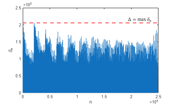
maxDelta = max(delta)

maxDelta = single

2.0559e+05

Depending on your requirements, maxDelta may or may not be small enough for the network to be considered stable.

Verify Local Stability of Network Output Classes

To evaluate the stability of the network classification, first calculate the network output at the center of each hypercuboid. If you know the ground truth at the center of each hypercuboid, then you can verify the network robustness by specifying labels as the ground truth labels.

xn = (xUpper+xLower)/2;
yn = minibatchpredict(net,xn,MiniBatchSize=4096);
labels = scores2label(yn,helpers.classNames);

Next, verify whether the class label changes within the hypercuboid by using the verifyNetworkRobustness function, as described in Verify Local Robustness of ACAS Xu Neural Networks.

[results,detailedResults] = verifyNetworkRobustness(net,xLower,xUpper, labels,ExecutionEnvironment=executionEnvironment,Verbose=true,MiniBatchSize=4096);

Number of mini-batches to process: 61
..........   ..........   ..........   ..........   .......... (50 mini-batches)
..........   .                                                 (61 mini-batches)
Total time = 16.1 seconds.

summary(results,Statistics="counts")

results: 248832×1 categorical

     verified       88334 
     violated           0 
     unproven      160498

Compute the proportion of the ODD that is verified as stable under this regular tiling prescription. The hypercuboids do not overlap, all have the same volume, and cover the entire ODD. Therefore, simply compute the proportion of results that are "verified".

verifiedProportion = sum(results == "verified") / numel(results)

verifiedProportion = 
0.3550

Compute the proportion of the ODD that predicts each class in the verified regions.

verifiedLabels = labels(results=="verified");
classPredictionCount = summary(verifiedLabels).Counts

classPredictionCount = 1×5

    88334    0    0    0    0

numHypercuboids = length(results);
unverifiedCount = numHypercuboids - sum(classPredictionCount);

Plot the results in a bar chart.

figure
b = bar([helpers.classNames; "Unverified"],...
    [classPredictionCount unverifiedCount]/numHypercuboids);
ylim([0 1])
title("Proportion of ODD by Class")

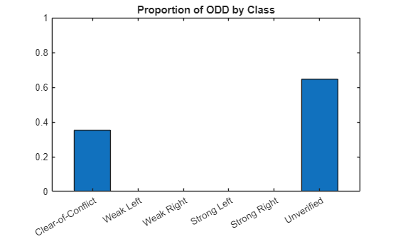
The figure shows that the most stable region of the ODD predicts Clear-of-Conflict. To reduce the number of hypercuboids that are unverified, increase numHypercuboidsPerDimension and rerun the analysis.

Verify Global Stability Using Overlapping Hypercuboids

A neural network is globally stable across the entire ODD if the network is locally stable at every element of the ODD.

$\forall x_{i}, x_{j}, \in D | x_{i} - x_{j} |_{\infty} \leq ϵ \to | f (x_{i}) - f (x_{j}) |_{\infty} \leq δ$ .

To verify global stability across the entire ODD, it is not enough to verify local stability at the center of each hypercuboid, because two points could be less than $ϵ$ apart, but located in different hypercuboids.

One approach to verifying global stability is to use more than one tessellation of the ODD, such that for each pair of points $x_{i}$ and $x_{j}$ less than $ϵ$ apart in the ODD, there is at least one local hypercuboid that contains both. You can use the estimateNetworkOutputBounds function for all local hypercuboids, across all tessellations of the ODD, and compute the maximum $| y_{u} - y_{l} |_{\infty}$ , which is an upper bound on the true $δ$ .

Create the tessellations by moving the original lattice towards each face center and each corner of the surrounding hypercuboid. Do not include equivalent lattices. For example, moving half a lattice constant to the right creates the same lattice as moving half a lattice constant to the left.

For example, in 2-D, you can use $2^{2} = 4$ lattices:

The original lattice.
Shift right — A lattice that, compared to the original lattice, shifts half a lattice constant to the right, in the direction (0,1).
Shift up — A lattice that, compared to the original lattice, shifts half a lattice constant to the top, in the direction (1,0).
Shift right and up — A lattice that, compared to the original lattice, shifts half a lattice constant to the right and half a lattice constant to the top, in the direction (1,1).

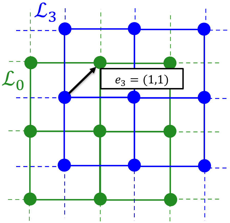
In 5-D, use $2^{5} = 32$ 5-D lattices, shifted relative to the original lattice in directions $e_{1} = (1, 0, 0, 0, 0)$ , $e_{2} = (0, 1, 0, 0, 0)$ , ..., $e_{31} = (1, 1, 1, 1, 1)$ .

First, construct these lattices using the latticeSet function, which is defined at the bottom of this example.

[xLower,xUpper] = latticeSet(inputRange,numHypercuboidsPerDimension);

Calculate the output range for each hypercuboid in each lattice by using the estimateNetworkOutputBounds function.

xLower = cat(2, xLower{:});
xUpper = cat(2, xUpper{:});
[yLower,yUpper] = estimateNetworkOutputBounds(net,xLower,xUpper,ExecutionEnvironment=executionEnvironment,Verbose=true,MiniBatchSize=4096);

Number of mini-batches to process: 1572
..........   ..........   ..........   ..........   .......... (50 mini-batches)
..........   ..........   ..........   ..........   .......... (100 mini-batches)
..........   ..........   ..........   ..........   .......... (150 mini-batches)
..........   ..........   ..........   ..........   .......... (200 mini-batches)
..........   ..........   ..........   ..........   .......... (250 mini-batches)
..........   ..........   ..........   ..........   .......... (300 mini-batches)
..........   ..........   ..........   ..........   .......... (350 mini-batches)
..........   ..........   ..........   ..........   .......... (400 mini-batches)
..........   ..........   ..........   ..........   .......... (450 mini-batches)
..........   ..........   ..........   ..........   .......... (500 mini-batches)
..........   ..........   ..........   ..........   .......... (550 mini-batches)
..........   ..........   ..........   ..........   .......... (600 mini-batches)
..........   ..........   ..........   ..........   .......... (650 mini-batches)
..........   ..........   ..........   ..........   .......... (700 mini-batches)
..........   ..........   ..........   ..........   .......... (750 mini-batches)
..........   ..........   ..........   ..........   .......... (800 mini-batches)
..........   ..........   ..........   ..........   .......... (850 mini-batches)
..........   ..........   ..........   ..........   .......... (900 mini-batches)
..........   ..........   ..........   ..........   .......... (950 mini-batches)
..........   ..........   ..........   ..........   .......... (1000 mini-batches)
..........   ..........   ..........   ..........   .......... (1050 mini-batches)
..........   ..........   ..........   ..........   .......... (1100 mini-batches)
..........   ..........   ..........   ..........   .......... (1150 mini-batches)
..........   ..........   ..........   ..........   .......... (1200 mini-batches)
..........   ..........   ..........   ..........   .......... (1250 mini-batches)
..........   ..........   ..........   ..........   .......... (1300 mini-batches)
..........   ..........   ..........   ..........   .......... (1350 mini-batches)
..........   ..........   ..........   ..........   .......... (1400 mini-batches)
..........   ..........   ..........   ..........   .......... (1450 mini-batches)
..........   ..........   ..........   ..........   .......... (1500 mini-batches)
..........   ..........   ..........   ..........   .......... (1550 mini-batches)
..........   ..........   ..                                   (1572 mini-batches)
Total time = 480.7 seconds.

The maximum output difference $δ$ for two points inside the range from xLower to xUpper is the distance between yLower and yUpper.

delta = vecnorm(extractdata(yUpper-yLower),Inf);

Plot $δ$ for each hypercuboid using the plotDelta function, defined at the bottom of this example.

plotDelta(delta);

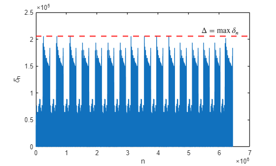
maxDelta = max(delta)

maxDelta = single

2.0559e+05

Depending on your requirements, maxDelta may or may not be small enough for the network to be considered stable.

Close the parallel pool.

delete(gcp("nocreate"));

Supporting Functions

`uniformLattice`

The uniformLattice function creates lower and upper vertices for each hypercuboid in the uniform lattice, returned as dlarray objects with format "BC".

function [xLower,xUpper] = uniformLattice(inputRange,numHypercuboidsPerDimension)
globalLowerBound = inputRange(:,1);
globalUpperBound = inputRange(:,2);

% Number of dimensions of the ODD
ndims = 5;

% Create a uniform 5-D lattice between [0 0 0 0 0] and [1 1 1 1 1]
latticeNodes = cell(1,ndims);
[latticeNodes{:}] = ndgrid(linspace(0,1,numHypercuboidsPerDimension+1));

% Rescale the lattice to lie between globalLowerBound and globalUpperBound
scale = globalUpperBound - globalLowerBound;
offset = globalLowerBound;
for ii = 1:ndims
    latticeNodes{ii} = latticeNodes{ii} * scale(ii) + offset(ii);
end

% Return the lower and upper bounds of each hypercuboid
numHypercuboids = prod(size(latticeNodes{1})-1);
xLower = dlarray(zeros(numHypercuboids,5),"BC");
xUpper = dlarray(zeros(numHypercuboids,5),"BC");

for ii = 1:ndims
    lowerNodes = latticeNodes{ii}(1:end-1,1:end-1,1:end-1,1:end-1,1:end-1);
    upperNodes = latticeNodes{ii}(2:end,2:end,2:end,2:end,2:end);
    xLower(ii,:) = lowerNodes(:);
    xUpper(ii,:) = upperNodes(:);
end
end

`latticeSet`

The latticeSet function returns the lower and upper vertices for each hypercuboid in each of the $2^{5} = 32$ 5-D lattices.

function [xLower,xUpper] = latticeSet(inputRange,numHypercuboidsPerDimension)

% Create a container for the lattices
xLower = cell(32,1);
xUpper = cell(32,1);

% Create initial lattice
[xLower{32}, xUpper{32}] = uniformLattice(inputRange,numHypercuboidsPerDimension);
epsilon = ( inputRange(:,2) - inputRange(:,1) )' / numHypercuboidsPerDimension;

% Create L_k
for ii = 1:31
translationVector = latticeTranslationVector(ii);
xLowerTranslated = xLower{32} + (translationVector.*epsilon)';
xUpperTranslated = xUpper{32} + (translationVector.*epsilon)';
% Remove tiles that exceed the ODD - these will be by the upper bounds
% since positive translation in all dimensions
xLowerTranslated(:,any(xUpperTranslated > inputRange(:,2),1)) = [];
xUpperTranslated(:,any(xUpperTranslated > inputRange(:,2),1)) = [];
xLower{ii} = xLowerTranslated;
xUpper{ii} = xUpperTranslated;
end
end

`latticeTranslationVector`

The latticeTranslationVector function creates the i-th of the 31 5-D lattice translation vectors by using the bitget function to obtain the inverted base 2 encoding of i as a vector. For example:

>> latticeTranslationVector(1)
[1 0 0 0 0]
>> latticeTranslationVector(25)
[1 0 0 1 1]

function v = latticeTranslationVector(i)
    v = bitget(i,1:5);
end

`plotDelta`

The plotDelta function plots the maximum estimated output bound range for each hypercuboid.

function plotDelta(delta)
figure
plot(delta)
hold on
yline(max(delta),'r--',LineWidth=2)
xlabel("n")
ylabel("\delta_n")
x_lim = xlim;

x_pos = x_lim(2)*0.95;
y_pos = max(delta);
text(x_pos, y_pos, "$$\Delta = \max\,\delta_n$$", ...
    Interpreter="latex", ...
    HorizontalAlignment="right", ...
    VerticalAlignment="bottom", ...
    FontSize=12, ...
    BackgroundColor="white");
end