Train Network with Complex-Valued Data
This example shows how to predict the frequency of a complex-valued waveform using a 1-D convolutional neural network.
To pass complex-valued data to a neural network, you can use the input layer to split the complex values into their real and imaginary parts before it passes the data to the subsequent layers in the network. When the input layer splits the input data in this way, the layer outputs the split data as extra channels. This diagram shows how complex-valued data flows through a convolutional neural network.
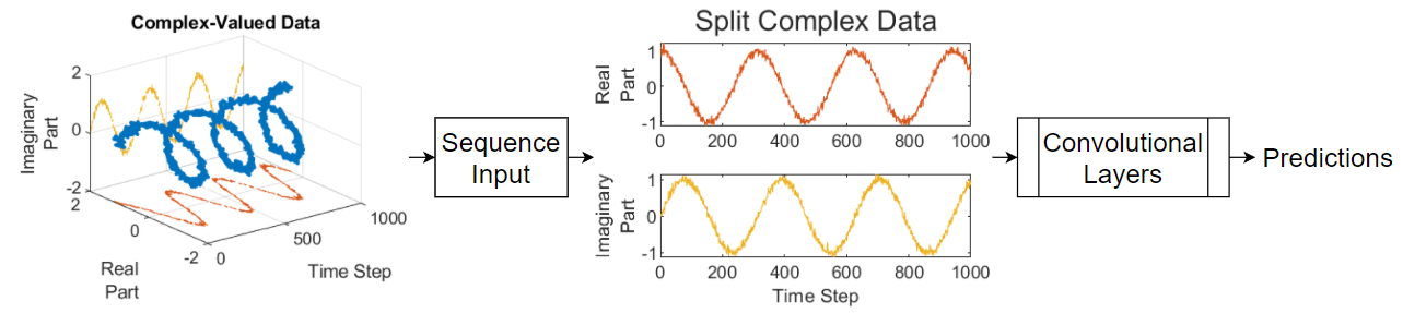
To split the complex-valued data into its real and imaginary parts as its input to a network, set the SplitComplexInputs option of the network input layer to 1 (true).
This example trains a sequence-to-one regression network using the Complex Waveform data set, which contains 500 synthetically generated complex-valued waveforms of varying lengths with two channels. The network trained in this example predicts the frequency of the waveforms.
For an example showing how to train a complex-valued neural network to make predictions on complex-valued data without first splitting the data into real and imaginary parts, see Denoise Complex-Valued Signal Using Multilayer Perceptron.
Load Sequence Data
Load the example data from ComplexWaveformData.mat. The data is a numObservations-by-1 cell array of sequences, where numObservations is the number of sequences. Each sequence is a numChannels-by-numTimeSteps complex-valued array, where numChannels is the number of channels of the sequence and numTimeSteps is the number of time steps in the sequence. The corresponding targets are in a numObservations-by-numResponses numeric array of the frequencies of the waveforms, where numResponses is the number of channels of the targets.
load ComplexWaveformDataView the number of observations.
numObservations = numel(data)
numObservations = 500
View the sizes of the first few sequences and the corresponding frequencies.
data(1:4)
ans=4×1 cell array
    {2×157 double}
    {2×112 double}
    {2×10² double}
    {2×146 double}
freq(1:4,:)
ans = 4×1

    5.6232
    2.1981
    4.6921
    4.5805
View the number of channels of the sequences. For network training, each sequence must have the same number of channels.
numChannels = size(data{1},1)numChannels = 2
View the number of responses (the number of channels of the targets).
numResponses = size(freq,2)
numResponses = 1
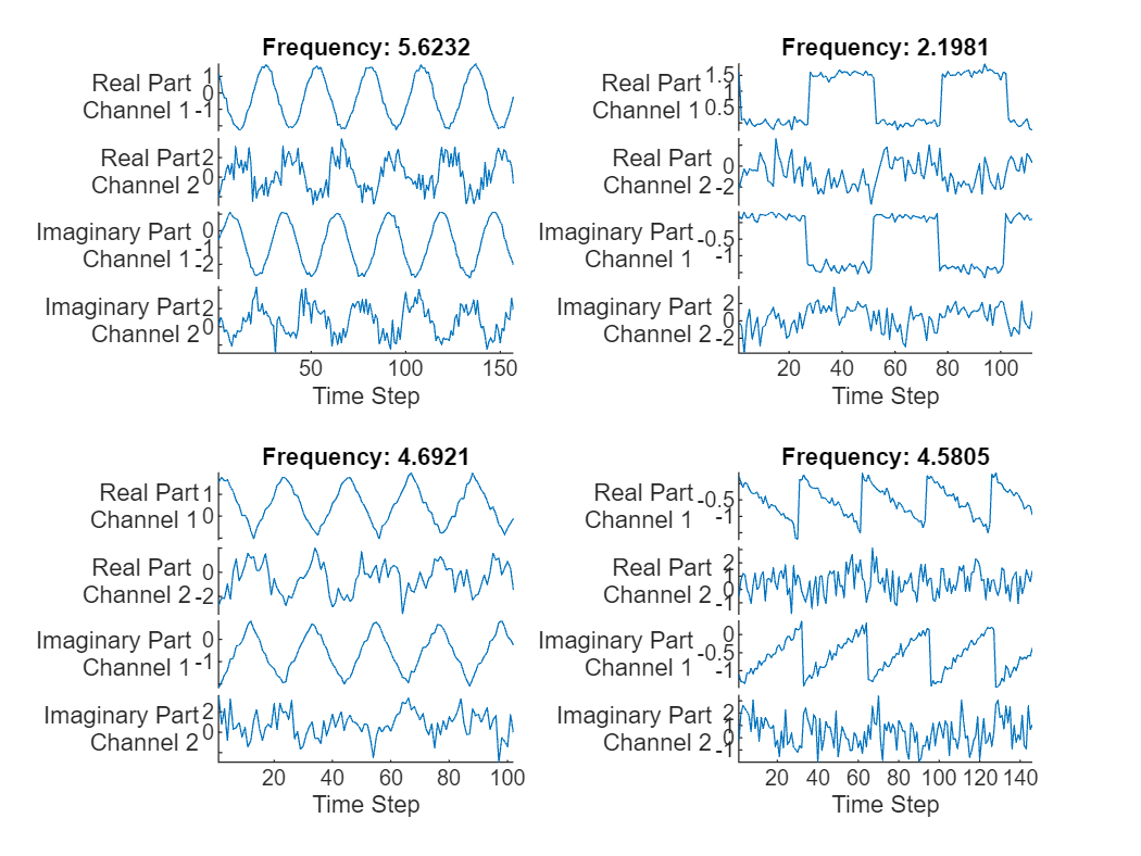
Visualize the first few sequences in plots.
displayLabels = [ ...
    "Real Part" + newline + "Channel " + string(1:numChannels), ...
    "Imaginary Part" + newline + "Channel " + string(1:numChannels)];

figure
tiledlayout(2,2)
for i = 1:4
    nexttile

    stackedplot([real(data{i}') imag(data{i}')],DisplayLabels=displayLabels)

    xlabel("Time Step")
    title("Frequency: " + freq(i))
end
Prepare Data for Training
Set aside data for validation and testing. Partition the data into a training set containing 80% of the data, a validation set containing 10% of the data, and a test set containing the remaining 10% of the data. To partition the data, use the trainingPartitions function, attached to this example as a supporting file. To access this file, open the example as a live script.
[idxTrain,idxValidation,idxTest] = trainingPartitions(numObservations, [0.8 0.1 0.1]);

XTrain = data(idxTrain);
XValidation = data(idxValidation);
XTest = data(idxTest);

TTrain = freq(idxTrain);
TValidation = freq(idxValidation);
TTest = freq(idxTest);
To help check the network is valid for the shorter training sequences, you can pass the length of the shortest sequence to the sequence input layer of the network. Calculate the length of the shortest training sequence.
for n = 1:numel(XTrain)
    sequenceLengths(n) = size(XTrain{n},2);
end
minLength = min(sequenceLengths)
minLength = 76
Define 1-D Convolutional Network Architecture
Define the 1-D convolutional neural network architecture.
Specify a sequence input layer with input size matching the number of features of the input data.
To split the input data into its real and imaginary parts, set the
SplitComplexInputsoption of the input layer to1(true).To help check the network is valid for the shorter training sequences, set the
MinLengthoption to the length of the shortest training sequence.Specify two blocks of 1-D convolution, ReLU, and layer normalization layers, where the convolutional layer has a filter size of 5. Specify 32 and 64 filters for the first and second convolutional layers, respectively. For both convolutional layers, left-pad the inputs such that the outputs have the same length (causal padding).
To reduce the output of the convolutional layers to a single vector, use a 1-D global average pooling layer.
To specify the number of values to predict, include a fully connected layer with a size matching the number of responses.
filterSize = 5;
numFilters = 32;

layers = [ ...
    sequenceInputLayer(numChannels,SplitComplexInputs=true,MinLength=minLength)
    convolution1dLayer(filterSize,numFilters,Padding="causal")
    reluLayer
    layerNormalizationLayer
    convolution1dLayer(filterSize,2*numFilters,Padding="causal")
    reluLayer
    layerNormalizationLayer
    globalAveragePooling1dLayer
    fullyConnectedLayer(numResponses)];
Specify Training Options
Specify the training options.
Train using the Adam optimizer.
Specify that the input data has format
"CTB"(channel, time, batch).Train for 250 epochs. For larger data sets, you might not need to train for as many epochs for a good fit.
Specify the sequences and responses used for validation.
Output the network that gives the lowest validation loss.
Display the training process in a plot.
Disable the verbose output.
options = trainingOptions("adam", ...
    InputDataFormats="CTB", ...
    MaxEpochs=250, ...
    ValidationData={XValidation, TValidation}, ...
    OutputNetwork="best-validation-loss", ...
    Plots="training-progress", ...
    Verbose=false);
Train Network
Train the neural network using the trainnet function. For regression, use mean squared error loss. By default, the trainnet function uses a GPU if one is available. Using a GPU requires a Parallel Computing Toolbox™ license and a supported GPU device. For information on supported devices, see GPU Computing Requirements (Parallel Computing Toolbox). Otherwise, the function uses the CPU. To specify the execution environment, use the ExecutionEnvironment training option.
net = trainnet(XTrain,TTrain,layers,"mse",options);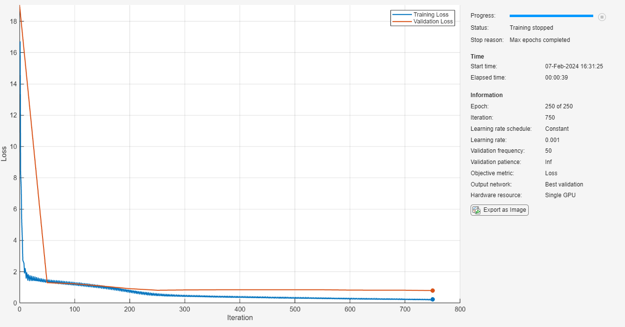
Test Network
Make predictions with the test data using the minibatchpredict function. By default, the minibatchpredict function uses a GPU if one is available. Left-pad the data and specify that it has format "CTB" (channel, time, batch).
YTest = minibatchpredict(net,XTest, ...
    SequencePaddingDirection="left", ...
    InputDataFormats="CTB");
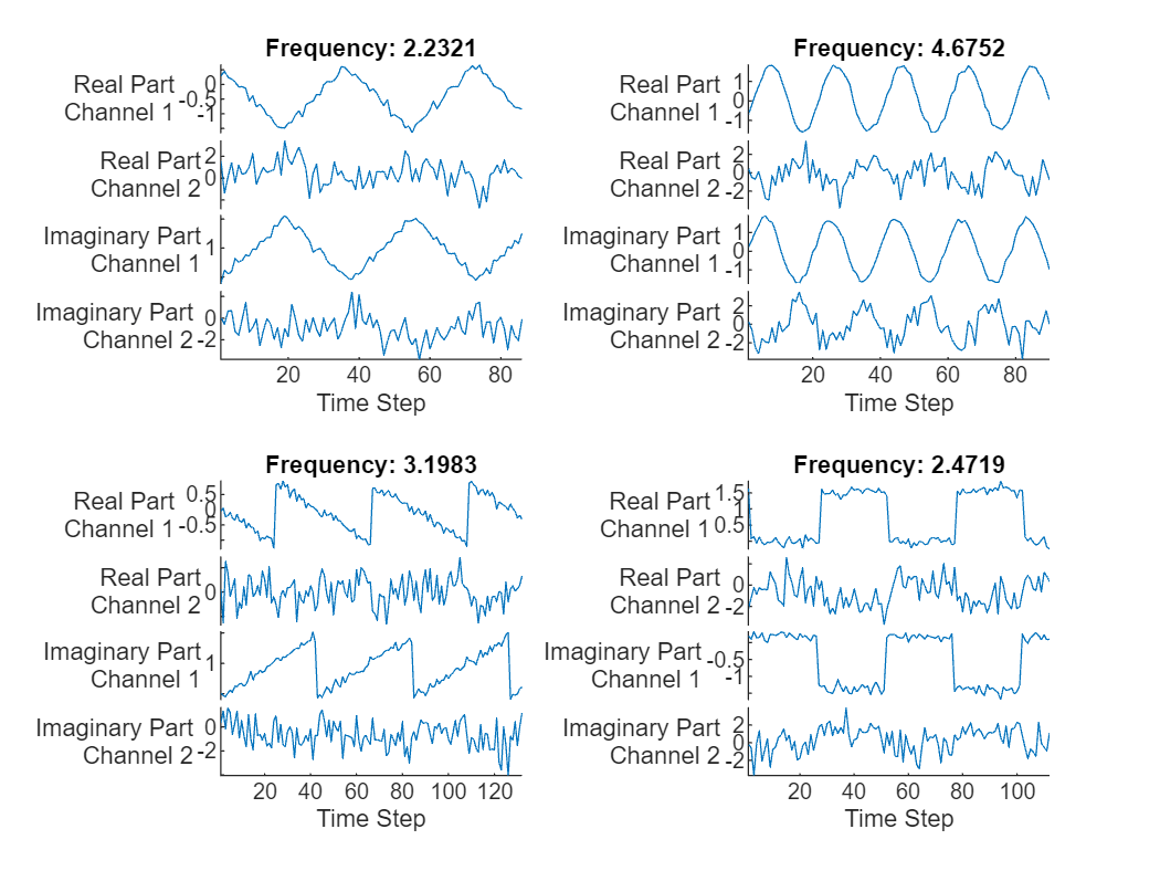
Visualize the first few predictions in a plot.
displayLabels = [ ...
    "Real Part" + newline + "Channel " + string(1:numChannels), ...
    "Imaginary Part" + newline + "Channel " + string(1:numChannels)];

figure
tiledlayout(2,2)
for i = 1:4
    nexttile

    stackedplot([real(XTest{i}') imag(XTest{i}')], DisplayLabels=displayLabels);

    xlabel("Time Step")
    title("Frequency: " + YTest(i))
end
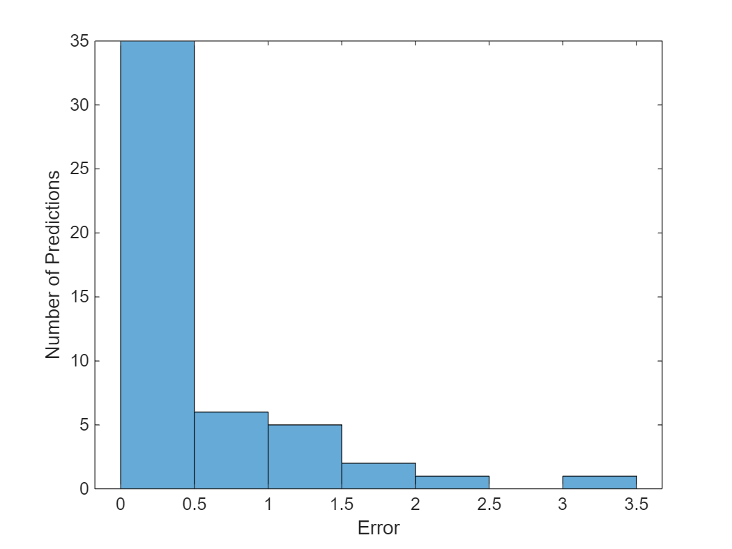
Visualize the mean squared errors in a histogram.
figure
histogram(mean((TTest - YTest).^2,2))
xlabel("Error")
ylabel("Number of Predictions")
Calculate the overall root mean squared error.
rmse = sqrt(mean((YTest-TTest).^2))
rmse = single
    0.6751
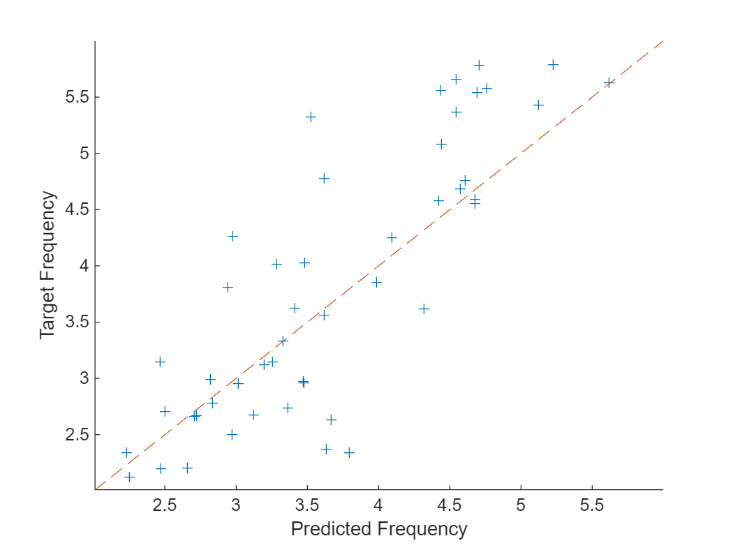
Plot the predicted frequencies against the target frequencies.
figure
scatter(YTest,TTest,"+");
xlabel("Predicted Frequency")
ylabel("Target Frequency")
hold on

m = min(freq);
M = max(freq);
xlim([m M])
ylim([m M])
plot([m M], [m M], "--")
See Also
trainnet | trainingOptions | dlnetwork | testnet | minibatchpredict | predict | scores2label | convolution1dLayer | sequenceInputLayer