Reduced Order Modeling Using Continuous-Time Echo State Network

This example shows how to train a continuous-time echo state network (CTESN) model to solve Robertson's equation.

An echo state network (ESN) is a reservoir computing framework that projects signals from higher dimensional spaces defined by the dynamics of a fixed nonlinear system called a reservoir [1, 2]. A continuous-time echo state network (CTESN) is a variant of an ESN that supports an underlying adaptive time process and avoids issues when it computes gradients during training [1].

If you need to solve an ODE in a model multiple times with different parameters, then to save computational resources, instead of approximating the solution using an ODE solver within the system, you can train a neural network using a collection of automatically generated solutions and then incorporate the neural network in your model. A CTESN model typically evaluates faster than an ODE solver.

This example trains a CTESN model to solve the Robertson equation, which is a system of ODEs that models the concentration of chemicals in a reaction.

Define Model

The Robertson equation is a system of three ODEs that model the concentrations of chemicals in a reaction. The parameterized form of this equation is given by:

$$\begin{array}{l}\frac{d{y}_1}{dt}=-p_1{y}_1+p_3{y}_2{y}_3\\ \frac{d{y}_2}{dt}=p_1{y}_1-p_3{y}_2{y}_3-p_2{y}_2^2\\ \frac{d{y}_3}{dt}=p_2{y}_2^2\end{array}$$

where $$y_1$$, $$y_2$$, and $$y_3$$ are functions of $$t$$, $$p=(p_1,p_2,p_3)\in \mathbb{R}$$ are parameters, and the ODE has initial condition $$y_0=(1,0,0)$$.

Define the robertson function, listed in the Robertson Equation ODE Function section of the example, that takes as input the ODE inputs $$t$$ (unused) the ODE solutions $$y=(y_1,y_2,y_3)$$, and the ODE parameters $$p$$ and outputs the derivatives $$\frac{d{y}_1}{dt}$$, $$\frac{d{y}_2}{dt}$$, and $$\frac{d{y}_3}{dt}$$.

Generate Training Data

Use the ode15s ODE solver to generate training data. Generate a set of input parameters pTrain and the corresponding ODE solutions yTrain.

Solve the ODE on the time interval $$[0,10^5]$$ with initial condition $$y(0)=(1,0,0)$$.

tspan = [0 1e5];
y0 = [1 0 0];

Randomly sample 100 values for pTrain, where the parameters are in the space $$[0.9p_{0,1},1.1p_{0,1}]\times [0.9p_{0,2},1.1p_{0,2}]\times [0.9p_{0,3},1.1p_{0,3}]$$, where $$p_0=(0.04,3\times 10^7,10^4)$$.

p0 = [0.04 3e7 1e4]';
numObservationsTrain = 100;
m = 0.9 * p0;
M = 1.1 * p0;
pTrain = m + (M-m).*rand(numel(p0),numObservationsTrain);

Solve the ODE system on the training parameter space to create training data. The Robertson equation is a stiff system, so the ode15s function is well suited.

The ode15s function requires a ODE function with two inputs. For each observation, use an anonymous function to parameterize the robertson function with the corresponding parameters in pTrain to have two inputs.

tTrain = cell(numObservationsTrain,1);
yTrain = cell(numObservationsTrain,1);

for n = 1:numObservationsTrain
    fcn = @(t,u) robertson(t,u,pTrain(:,n));
    [t,y] = ode15s(fcn,tspan,y0);
    tTrain{n} = t;
    yTrain{n} = y;
end

View the sizes of the first few observations. The time steps are vectors of time step values. The ODE solutions are $$T$$-by-$$C$$ matrices, where $$T$$ is the number of time steps of the sequence and $$C$$ is the output size.

head(tTrain)

    {123x1 double}
    {121x1 double}
    {114x1 double}
    {120x1 double}
    {120x1 double}
    {114x1 double}
    {118x1 double}
    {120x1 double}

head(yTrain)

    {123x3 double}
    {121x3 double}
    {114x3 double}
    {120x3 double}
    {120x3 double}
    {114x3 double}
    {118x3 double}
    {120x3 double}

Define CTESN Model

A CTESN models an ODE system using a reservoir system in a latent space.

In particular, given the parameterized system

$$\frac{d{y}_p}{dt}=f_p(t,y)$$

where $$p$$ denotes a set of parameters, the reservoir system is defined by

$$\begin{array}{l}\frac{dr}{dt}=\tanh (Ar+V{y}_{p_{\ast }})\\ {\underset{}{\overset{\sim }{y}}}_p(t)=r(t)W_p\end{array}$$

where

• $$p_{\ast }$$ denotes a set of parameters with known solution $$y_{p_{\ast }}$$.

• $${\underset{}{\overset{\sim }{y}}}_p$$ denotes the model approximation of the targets $$y_p$$.

• $$r\in {\mathbb{R}}^{N_R}$$ is the reservoir state with reservoir dimension $$N_R$$.

• $$A\in {\mathbb{R}}^{N_R\times N_R}$$ and $$V\in {\mathbb{R}}^{N_R\times N}$$ are random matrices and $$N$$ is the size of $$y$$.

• $$W_p\in {\mathbb{R}}^{N\times N_R}$$ is the trained output matrix.

Define the reservoir function, listed in the Reservoir System ODE Function section of the example, that takes as input a time step t, the reservoir state, an interpolant that evaluates $$y_{p_{\ast }}$$ for a specified time $$t$$, and random matrices A and V, and outputs the derivative dr that satisfies the ODE system.

Specify the dimension of the reservoir system and the density of the sparse random matrix A.

reservoirDimension = 200;
density = 0.01;

Train CTESN Model

The CTESN model is characterized by the reservoir $$r$$ and the matrix $$W_p$$. The CTESN model uses the same reservoir $$r$$ for any value of $$p$$. For an input $$p$$, the model predicts the solution $$y_p$$ using the equation $$y_p(t)=r(t)W_p$$, where $$r$$ is the reservoir and $$W_p$$ is the output of the radial basis network.

Solve Reservoir System

Initialize the reservoir system and sparse reservoir matrix.

outputSize = numel(y0);
A = sprandn(reservoirDimension,reservoirDimension,density);
V = randn(reservoirDimension,outputSize);

To allow the ODE solver of the reservoir system to evaluate $$y_{p_{\ast }}(t)$$ for arbitrary time $$t$$, choose an arbitrary parameter sample as $$p_{\ast }$$ and fit an interpolation to $$y_{p_{\ast }}(t)$$ from the ode15s solution for that parameter. Create a gridded data interpolant for $$y_{p_{\ast }}$$ using the first training observation.

tpStar = tTrain{1};
ypStar = yTrain{1};
ypStarInterpolant = griddedInterpolant(tpStar,ypStar,"spline");

Solve the reservoir system for $$p_{\ast }$$. The reservoir system is not stiff so the fast solver ode23 is well suited.

fcn = @(t,r) reservoir(t,r,ypStarInterpolant,A,V);
r0 = zeros(reservoirDimension,1);
[tr,r] = ode23(fcn,tspan,r0);

To introduce a bias term to the linear output $$r(t)W_p$$, add a column of ones to the reservoir state.

r(:,end+1) = 1;

Create an interpolant for $$r$$.

rInterpolant = griddedInterpolant(tr,r,"spline")

rInterpolant = 
  griddedInterpolant with properties:

            GridVectors: {[8683x1 double]}
                 Values: [8683x201 double]
                 Method: 'spline'
    ExtrapolationMethod: 'spline'

Train Radial Basis Network

Train a radial basis neural network that maps $$p$$ to the matrix $$W_p$$, where $$W$$ is a learned matrix.

This diagram shows the structure of a radial bias network.

The network has three layers:

• The feature input layer inputs data to the network as 2-D arrays with dimensions corresponding to channels and observations.

• The radial basis layer maps its input to the vector $$exp(-d^2)$$, where $$d$$ is the weighted distance between its input and its centroids with weight given by $$\frac{1}{S}\sqrt{\log (2)}$$, where $$S$$ denotes the spread.

• The linear layer applies a transformation $$Ax+b$$, where $$A$$ and $$b$$ are fixed parameters (that is, they are not learnable parameters).

Fit an exact radial basis network using the trainExactRadialBasisNetwork example function, attached to this example as a supporting file. To access this file, open the example as a live script.

The function

• Sets the radial basis layer centroids to pTrain.

• Fits the linear layer weights using linear regression using the outputs of the radial basis layer as predictors and yTrain as the targets.

net = trainExactRadialBasisNetwork(tTrain,yTrain,pTrain,tr,r,Spread=0.1)

net = 
  dlnetwork with properties:

         Layers: [3x1 nnet.cnn.layer.Layer]
    Connections: [2x2 table]
     Learnables: [0x3 table]
          State: [0x3 table]
     InputNames: {'input'}
    OutputNames: {'linear'}
    Initialized: 1

  View summary with summary.

Test Model

To test the model, compare the predicted outputs with the outputs from an ODE solver for a set of previously unseen input parameters.

Create an array of time steps and a set of previously unseen parameters.

tTest = linspace(tspan(1),tspan(2),1e4);
p0Test = [0.041 3.1e7 1.02e4]';

Calculate the targets TTest by solving the ODE using the ODE solver ode15s with the time steps tTest and initial conditions y0.

fcn = @(t,y) robertson(t,y,p0Test);
[~,TTest] = ode15s(fcn,tTest,y0);

For the specified time steps and parameters predict the values of $$y$$ using the modelPredictions function, listed in the Model Predictions Function section of the example. To access this function, open the example as a live script.

p0Test = dlarray(p0Test,"CB");
yTest = modelPredictions(net,rInterpolant,outputSize,tTest,p0Test);

Calculate the mean squared error between the predictions and the targets.

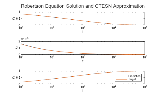
err = mean((yTest-TTest).^2,"all")

err = 
3.0084e-06

Plot the predictions and targets with the time steps in logarithmic scale.

figure
layout = tiledlayout(outputSize,1);
title(layout,"Robertson Equation Solution and CTESN Approximation");
for i = 1:outputSize
    nexttile

    semilogx(tTest,yTest(:,i),"--");

    hold on
    semilogx(tTest,TTest(:,i))

    xlabel("t")
    ylabel("y_" + i)
end
legend(["Prediction" "Target"])

Compare Performance

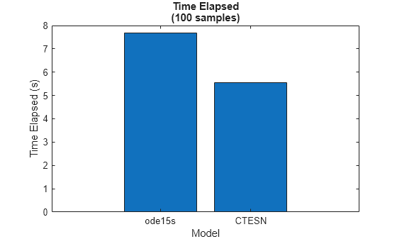
For 100 random sets of parameters, measure the time it takes to evaluate the ODE solutions using an ODE solver and a CTESN model.

Generate 100 random sets of parameters.

numSamples = 100;
pTest = (0.9 + 0.2*rand(outputSize,numSamples)).*p0;

Measure the time taken to solve the ODE system using the ode15s ODE solver.

tic
for n = 1:numSamples
    p = pTest(:,n);
    fcn = @(t,y) robertson(t,y,p);
    [~,y] = ode15s(fcn,tTest,y0);
end
elapsedODE15s = toc

elapsedODE15s = 
8.2300

Measure the time taken evaluating the CTESN model.

tic
pTest = dlarray(pTest,"CB");
for n = 1:numSamples
    p = pTest(:,n);
    yTest = modelPredictions(net,rInterpolant,outputSize,tTest,p);
end
elapsedCTESN = toc

elapsedCTESN = 
3.1410

Display the results in a bar chart.

figure
bar([elapsedODE15s elapsedCTESN])
xticklabels(["ode15s" "CTESN"])
xlabel("Model")
ylabel("Time Elapsed (s)")
title("Time Elapsed" + newline + "(" + numSamples + " samples)")

The bar chart shows the time elapsed for each model. For larger ODE systems, numbers of samples, or numbers of time steps, the CTESN model can be much faster than using an ODE solver directly.

Make Predictions Using New Data

Create an array of time steps and a set of parameters.

tNew = linspace(tspan(1),tspan(2),1e4);
pNew = [0.041 3.1e7 1.02e4]';

Make predictions using the modelPredictions function.

pNew = dlarray(pNew,"CB");
yNew = modelPredictions(net,rInterpolant,outputSize,tNew,pNew);

Display the predictions in a plot.

figure
layout = tiledlayout(3,1);
title(layout,"Predicted Values")
for i = 1:3
    nexttile
    semilogx(tNew,yNew(:,i),"--");
    xlabel("t")
    ylabel("y_"+i)
end

Supporting Functions

Robertson Equation ODE Function

The Robertson equation is a system of three ODEs that model the concentrations of chemicals in a reaction. The parameterized form of this equation can be written as

$$\begin{array}{l}\frac{d{y}_1}{dt}=-p_1{y}_1+p_3{y}_2{y}_3\\ \frac{d{y}_2}{dt}=p_1{y}_1-p_3{y}_2{y}_3-p_2{y}_2^2\\ \frac{d{y}_3}{dt}=p_2{y}_2^2\end{array}$$

where $$y_1$$, $$y_2$$, and $$y_3$$ are functions of $$t$$, $$p=(p_1,p_2,p_3)\in \mathbb{R}$$ are parameters, and the ODE has initial condition $$y_0=(1,0,0)$$.

The robertson function takes as input the ODE inputs $$t$$ (unused), $$y(t)=(y_1(t),y_2(t),y_3(t))$$, and the ODE parameters $$p$$, and outputs the derivatives.

function dy = robertson(~,y,p)

ax = p(1)*y(1);
cyz = p(3)*y(2)*y(3);
by2 = p(2)*(y(2)^2);

dy(1,1) = -ax + cyz;
dy(2,1) = ax - cyz - by2;
dy(3,1) = by2;

end

Reservoir System ODE Function

The reservoir function takes as input a time step t, the reservoir state r, an interpolant yInterpolant that evaluates $$y_{p_{\ast }}$$ for a specified time $$t$$, and random matrices A and V, and outputs the derivative dr that satisfies the ODE system given by

$$\frac{dr}{dt}=\tanh (Ar+V{y}_{p_{\ast }})$$

function dr = reservoir(t,r,yInterpolant,A,V)

dr = tanh(A*r + V*yInterpolant(t).');

end

Model Predictions Function

The modelPredictions function takes as input the radial basis network net, an interpolant rInterpolant that evaluates the reservoir for a specified time step, the output size outputSize, time steps t, and parameters p and outputs the solutions to the ODE system y.

function y = modelPredictions(net,rInterpolant,outputSize,t,p)

% Predict Wp.
WTest = predict(net,p);

% Calculate y = r*Wp.
numSamples = size(p,2);
WTest = reshape(WTest,[],outputSize,numSamples);
WTest = extractdata(WTest);
y = pagemtimes(rInterpolant(t),WTest);

end

References

[1] Ranjan Anatharaman, Yingbo Ma, Shashi Gowda, Chris Laughman, Viral Shah, Alan Edelman, Chris Rackauckas. "Accelerating Simulation of Stiff Nonlinear Systems using Continuous-Time Echo State Networks." Preprint, submitted October 7, 2020. https://arxiv.org/abs/2010.04004

[2] Ozturk, Mustafa C., Dongming Xu, and Jose C. Principe. "Analysis and design of echo state networks." Neural computation 19, no. 1 (2007): 111-138.