Choose Strategy for Exploring Experiment Parameters

When setting up an experiment in Experiment Manager, you can select a strategy for exploring your parameters. This table provides an overview of the available strategies to help you choose the most suitable one for your experiment.

Strategy	Description	When to Use
Exhaustive sweep	Evaluate all possible combinations of parameter values. The number of trials is the product of the number of possible values for each parameter.	Use this strategy when: Each parameter is represented with a discrete list of values. You have a manageable number of parameters and values. You do not need to examine the parameters outside of the list that you specify.
Random sampling (since R2025a)	Select parameter values based on probability distributions.	Use this strategy when: You have Statistics and Machine Learning Toolbox™. You want to specify the number of trials. You can describe each parameter with a probability distribution. You want to explore the parameter space without being restricted by the number of combinations.
Bayesian optimization	Iteratively improve parameter value selection based on the results from completed trials and the metric that you specify.	Use this strategy when: You have Statistics and Machine Learning Toolbox. Your experiment uses built-in training or custom training. You want Experiment Manager to automatically determine the best parameter values to try for each trial. You have a specific metric to optimize. You want to continue running trials until the maximum time or number of trials is reached. You want to optionally set different types of constraints for the optimization. Tip You can also use Bayesian optimization if you used the exhaustive sweep strategy to determine a reasonable range of values for each parameter, and now you want to use the Bayesian optimization strategy to explore that range.

Exhaustive Sweep

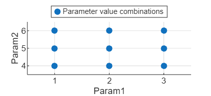
The exhaustive sweep strategy evaluates all possible combinations of parameter values.

For example, consider an experiment with two uncorrelated parameters: Param1, which has discrete values [1 2 3], and Param2, which has discrete values [4 5 6]. The exhaustive sweep strategy runs nine trials. This table and plot illustrate the exhaustive sweep strategy.

Param1	Param2
1	4
1	5
1	6
2	4
2	5
2	6
3	4
3	5
3	6

Configure Exhaustive Sweep Parameters

On the experiment definition tab, in the Parameters section, from the Strategy list, select Exhaustive Sweep. Then, in the table, specify these properties of the parameters.

• Name — Enter a parameter name that starts with a letter, followed by letters, digits, or underscores.

• Values — Specify a discrete set of values for each parameter as a numeric or logical scalar or vector, or as a string array, character vector, or cell array of character vectors.

For example, use the Add button to add two parameters to the table for an experiment using the exhaustive sweep strategy, and define the name and values for each parameter.

Random Sampling

Since R2025a

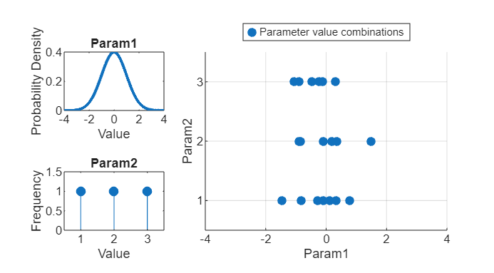
The random sampling strategy selects parameter values based on probability distributions.

For example, consider an experiment with a continuous parameter Param1 and a discrete parameter Param2. Represent Param1 using a normal distribution with a mean of 0 and a standard deviation of 1. Represent Param2 using a uniformly distributed multinomial distribution where the allowed values are 1, 2, and 3. The random sampling strategy randomly generates 20 parameter value combinations and runs 20 trials using those combinations. This table and plot illustrate the random sampling strategy.

Param1	Param2
0.53767	2
1.8339	1
–2.2588	3
0.86217	3
0.31877	3
–1.3077	3
–0.43359	3
0.34262	2
3.5784	2
2.7694	1
–1.3499	3
3.0349	1
0.7254	1
–0.063055	1
0.71474	1
–0.20497	3
–0.12414	3
1.4897	1
1.409	3
1.4172	1

Configure Random Sampling Parameters

On the experiment definition tab, in the Parameters section, from the Strategy list, select Random Sampling. Then, in the table, specify these properties of the parameters.

• Name — Enter a parameter name that starts with a letter, followed by letters, digits, or underscores.

• Distribution — Double-click the Distribution field and select a probability distribution from the list.

• Values — Set the value of each distribution property. To expand the view of a distribution and see its properties, click the arrow next to the distribution name.

For example, use the Add button to add two parameters to the table for an experiment using the random sampling strategy, and define the name, distribution, and distribution property values for each parameter.

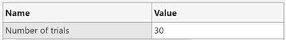
Then, optionally modify the number of trials to run for your experiment in the Random Sampling Options section.

Bayesian Optimization

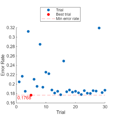
The Bayesian optimization strategy iteratively improves parameter value selection for built-in training or custom training experiments based on the results from completed trials and the metric that you specify.

For example, consider an experiment with four parameters. The Bayesian optimization strategy runs trials until finding the combination of parameter values that minimizes the error rate metric. This table and plot illustrate the Bayesian optimization strategy.

Trial	Error Rate
1	0.2050
2	0.2166
3	0.1848
4	0.3122
5	0.1768
6	0.2102
7	0.1954
8	0.2846
9	0.1934
10	0.2256
11	0.2224
12	0.1874
13	0.1814
14	0.1850
15	0.1775
16	0.2490
17	0.1838
18	0.1874
19	0.1832
20	0.1848
21	0.1818
22	0.1780
23	0.1860
24	0.1806
25	0.1804
26	0.1864
27	0.1852
28	0.3192
29	0.1822
30	0.1870

Configure Bayesian Optimization Parameters

On the experiment definition tab, in the Parameters section, from the Strategy list, select Bayesian Optimization. Then, in the table, specify these properties of the parameters.

• Name — Enter a parameter name that starts with a letter, followed by letters, digits, or underscores.

• Range — For a real- or integer-valued parameter, enter a two-element vector that specifies the lower bound and upper bound of the parameter. For a categorical parameter, enter an array of strings or a cell array of character vectors that lists the possible values of the parameter.

• Type — Double-click the Type field and select real for a real-valued parameter, integer for an integer-valued parameter, or categorical for a categorical parameter.

• Transform — Double-click the Transform field and select none to use no transformation or log to use a logarithmic transformation. If you select log, the parameter values must be positive. With this setting, the Bayesian optimization algorithm models the parameter on a logarithmic scale.

For example, use the Add button to add four parameters to the table for an experiment using the Bayesian optimization strategy, and define the name, range, type, and transform for each parameter.

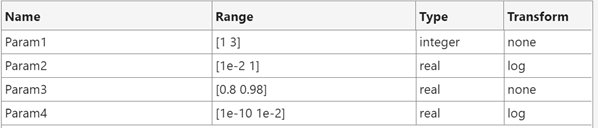
Next, optionally modify these options in the Post-Training Custom Metrics section.

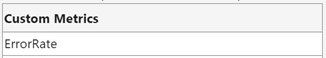
• Custom Metrics — Click the Add button to add a custom metric for Experiment Manager to compute after each trial is complete. Then, click Edit to edit the custom metric function in the MATLAB^® editor.

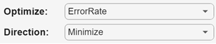
• Optimize — Choose a metric to optimize from the list. You can optimize a custom metric, the training or validation loss, or the training or validation accuracy or RMSE.

• Direction — Choose whether to minimize or maximize the metric that you selected in the Optimize field.

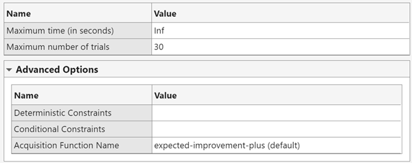
Then, optionally modify these options in the Bayesian Optimization Options section.

• Maximum time (in seconds) — Enter the maximum experiment duration in seconds. You can specify no maximum duration by entering Inf. The actual experiment duration can exceed this value because Experiment Manager checks this option only when a trial finishes executing.

• Maximum number of trials — Enter the maximum number of trials to run. The actual number of trials can exceed this value because Experiment Manager checks this option only when a trial finishes executing.

• Deterministic Constraints (since R2023a) — Enter the name of a deterministic constraint function. To run the Bayesian optimization algorithm without deterministic constraints, leave this option blank. For more information, see Deterministic Constraints — XConstraintFcn (Statistics and Machine Learning Toolbox).

• Conditional Constraints (since R2023a) — Enter the name of a conditional constraint function. To run the Bayesian optimization algorithm without conditional constraints, leave this option blank. For more information, see Conditional Constraints — ConditionalVariableFcn (Statistics and Machine Learning Toolbox).

• Acquisition Function Name (since R2023a) — Double-click the field and select an acquisition function from the list. The default value for this option is expected-improvement-plus. For more information, see Acquisition Function Types (Statistics and Machine Learning Toolbox).