How Dynamic Neural Networks Work
Feedforward and Recurrent Neural Networks
Dynamic networks can be divided into two categories: those that have only feedforward connections, and those that have feedback, or recurrent, connections. To understand the differences between static, feedforward-dynamic, and recurrent-dynamic networks, create some networks and see how they respond to an input sequence. (First, you might want to review Simulation with Sequential Inputs in a Dynamic Network.)
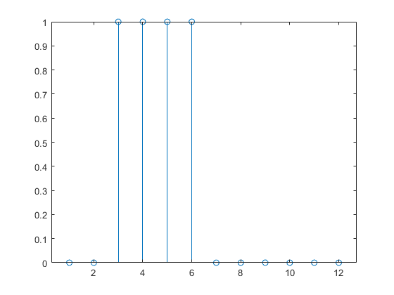
The following commands create a pulse input sequence and plot it:
p = {0 0 1 1 1 1 0 0 0 0 0 0};
stem(cell2mat(p))
Now create a static network and find the network response to the pulse sequence. The following commands create a simple linear network with one layer, one neuron, no bias, and a weight of 2:
net = linearlayer;
net.inputs{1}.size = 1;
net.layers{1}.dimensions = 1;
net.biasConnect = 0;
net.IW{1,1} = 2;

view(net)

You can now simulate the network response to the pulse input and plot it:
a = net(p);
stem(cell2mat(a))
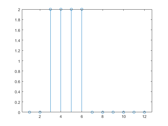
Note that the response of the static network lasts just as long as the input pulse. The response of the static network at any time point depends only on the value of the input sequence at that same time point.
Now create a dynamic network, but one that does not have any feedback connections (a nonrecurrent network). You can use the same network used in Simulation with Concurrent Inputs in a Dynamic Network, which was a linear network with a tapped delay line on the input:
net = linearlayer([0 1]);
net.inputs{1}.size = 1;
net.layers{1}.dimensions = 1;
net.biasConnect = 0;
net.IW{1,1} = [1 1];

view(net)

You can again simulate the network response to the pulse input and plot it:
a = net(p);
stem(cell2mat(a))
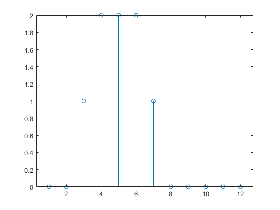
The response of the dynamic network lasts longer than the input pulse. The dynamic network has memory. Its response at any given time depends not only on the current input, but also on the history of the input sequence. If the network does not have any feedback connections, then only a finite amount of history will affect the response. In this figure you can see that the response to the pulse lasts one time step beyond the pulse duration. That is because the tapped delay line on the input has a maximum delay of 1.
Now consider a simple recurrent-dynamic network, shown in the following figure.
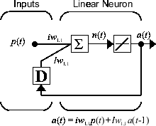
You can create the network, view it and simulate it with the following commands. The
narxnet command is discussed in Design Time Series NARX Feedback Neural Networks.
net = narxnet(0,1,[],'closed');
net.inputs{1}.size = 1;
net.layers{1}.dimensions = 1;
net.biasConnect = 0;
net.LW{1} = .5;
net.IW{1} = 1;
view(net)
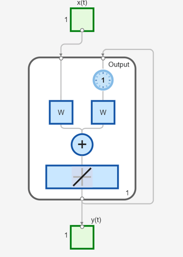
The following commands plot the network response.
a = net(p);
stem(cell2mat(a))

Notice that recurrent-dynamic networks typically have a longer response than feedforward-dynamic networks. For linear networks, feedforward-dynamic networks are called finite impulse response (FIR), because the response to an impulse input will become zero after a finite amount of time. Linear recurrent-dynamic networks are called infinite impulse response (IIR), because the response to an impulse can decay to zero (for a stable network), but it will never become exactly equal to zero. An impulse response for a nonlinear network cannot be defined, but the ideas of finite and infinite responses do carry over.
Applications of Dynamic Networks
Dynamic networks are generally more powerful than static networks (although somewhat more difficult to train). Because dynamic networks have memory, they can be trained to learn sequential or time-varying patterns. This has applications in such disparate areas as prediction in financial markets [RoJa96], channel equalization in communication systems [FeTs03], phase detection in power systems [KaGr96], sorting [JaRa04], fault detection [ChDa99], speech recognition [Robin94], and even the prediction of protein structure in genetics [GiPr02]. You can find a discussion of many more dynamic network applications in [MeJa00].
One principal application of dynamic neural networks is in control systems. This application is discussed in detail in Neural Network Control Systems. Dynamic networks are also well suited for filtering. You will see the use of some linear dynamic networks for filtering in and some of those ideas are extended in this topic, using nonlinear dynamic networks.
Dynamic Network Structures
The Deep Learning Toolbox™ software is designed to train a class of network called the Layered Digital Dynamic Network (LDDN). Any network that can be arranged in the form of an LDDN can be trained with the toolbox. Here is a basic description of the LDDN.
Each layer in the LDDN is made up of the following parts:
Set of weight matrices that come into that layer (which can connect from other layers or from external inputs), associated weight function rule used to combine the weight matrix with its input (normally standard matrix multiplication,
dotprod), and associated tapped delay lineBias vector
Net input function rule that is used to combine the outputs of the various weight functions with the bias to produce the net input (normally a summing junction,
netprod)Transfer function
The network has inputs that are connected to special weights, called input weights, and
denoted by IWi,j
(net.IW{i,j} in the code), where j denotes the number of
the input vector that enters the weight, and i denotes the number of the
layer to which the weight is connected. The weights connecting one layer to another are called
layer weights and are denoted by LWi,j
(net.LW{i,j} in the code), where j denotes the number of
the layer coming into the weight and i denotes the number of the layer at the
output of the weight.
The following figure is an example of a three-layer LDDN. The first layer has three weights associated with it: one input weight, a layer weight from layer 1, and a layer weight from layer 3. The two layer weights have tapped delay lines associated with them.
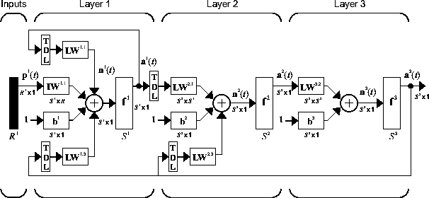
The Deep Learning Toolbox software can be used to train any LDDN, so long as the weight functions, net input functions, and transfer functions have derivatives. Most well-known dynamic network architectures can be represented in LDDN form. In the remainder of this topic you will see how to use some simple commands to create and train several very powerful dynamic networks. Other LDDN networks not covered in this topic can be created using the generic network command, as explained in Define Shallow Neural Network Architectures.
Dynamic Network Training
Dynamic networks are trained in the Deep Learning Toolbox software using the same gradient-based algorithms that were described in Multilayer Shallow Neural Networks and Backpropagation Training. You can select from any of the training functions that were presented in that topic. Examples are provided in the following sections.
Although dynamic networks can be trained using the same gradient-based algorithms that are used for static networks, the performance of the algorithms on dynamic networks can be quite different, and the gradient must be computed in a more complex way. Consider again the simple recurrent network shown in this figure.

The weights have two different effects on the network output. The first is the direct effect, because a change in the weight causes an immediate change in the output at the current time step. (This first effect can be computed using standard backpropagation.) The second is an indirect effect, because some of the inputs to the layer, such as a(t − 1), are also functions of the weights. To account for this indirect effect, you must use dynamic backpropagation to compute the gradients, which is more computationally intensive. (See [DeHa01a], [DeHa01b] and [DeHa07].) Expect dynamic backpropagation to take more time to train, in part for this reason. In addition, the error surfaces for dynamic networks can be more complex than those for static networks. Training is more likely to be trapped in local minima. This suggests that you might need to train the network several times to achieve an optimal result. See [DHH01] and [HDH09] for some discussion on the training of dynamic networks.
The remaining sections of this topic show how to create, train, and apply certain dynamic
networks to modeling, detection, and forecasting problems. Some of the networks require dynamic
backpropagation for computing the gradients and others do not. As a user, you do not need to
decide whether or not dynamic backpropagation is needed. This is determined automatically by the
software, which also decides on the best form of dynamic backpropagation to use. You just need
to create the network and then invoke the standard train command.