Design Time Series NARX Feedback Neural Networks
To see examples of using NARX networks being applied in open-loop form, closed-loop form and open/closed-loop multistep prediction see Multistep Neural Network Prediction.
Note
To design a NARX model, you can also use System Identification Toolbox™. This workflow is recommended because of these advantages:
Extend linear ARX models and model complex nonlinear behavior using flexible nonlinear functions such as wavelet networks, machine learning algorithms, and neural networks.
Include insights and physical information into your system by choosing appropriate regressors and starting with a linear model.
All the specific dynamic networks discussed so far have either been focused networks, with the dynamics only at the input layer, or feedforward networks. The nonlinear autoregressive network with exogenous inputs (NARX) is a recurrent dynamic network, with feedback connections enclosing several layers of the network. The NARX model is based on the linear ARX model, which is commonly used in time-series modeling.
The defining equation for the NARX model is
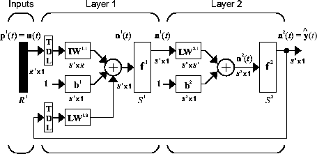
where the next value of the dependent output signal y(t) is regressed on previous values of the output signal and previous values of an independent (exogenous) input signal. You can implement the NARX model by using a feedforward neural network to approximate the function f. A diagram of the resulting network is shown below, where a two-layer feedforward network is used for the approximation. This implementation also allows for a vector ARX model, where the input and output can be multidimensional.

There are many applications for the NARX network. It can be used as a predictor, to predict the next value of the input signal. It can also be used for nonlinear filtering, in which the target output is a noise-free version of the input signal. The use of the NARX network is shown in another important application, the modeling of nonlinear dynamic systems.
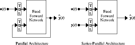
Before showing the training of the NARX network, an important configuration that is useful in training needs explanation. You can consider the output of the NARX network to be an estimate of the output of some nonlinear dynamic system that you are trying to model. The output is fed back to the input of the feedforward neural network as part of the standard NARX architecture, as shown in the left figure below. Because the true output is available during the training of the network, you could create a series-parallel architecture (see [NaPa91]), in which the true output is used instead of feeding back the estimated output, as shown in the right figure below. This has two advantages. The first is that the input to the feedforward network is more accurate. The second is that the resulting network has a purely feedforward architecture, and static backpropagation can be used for training.

The following shows the use of the series-parallel architecture for training a NARX network to model a dynamic system.
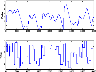
The example of the NARX network is the magnetic levitation system described beginning in Use the NARMA-L2 Controller Block. The bottom graph in the following figure shows the voltage applied to the electromagnet, and the top graph shows the position of the permanent magnet. The data was collected at a sampling interval of 0.01 seconds to form two time series.
The goal is to develop a NARX model for this magnetic levitation system.

First, load the training data. Use tapped delay lines with two delays for both the input and the output, so training begins with the third data point. There are two inputs to the series-parallel network, the u(t) sequence and the y(t) sequence.
[u,y] = maglev_dataset;
Create the series-parallel NARX network using the function narxnet. Use 10 neurons in the hidden layer and use trainlm for the training function, and then prepare the data with preparets:
d1 = [1:2];
d2 = [1:2];
narx_net = narxnet(d1,d2,10);
narx_net.divideFcn = '';
narx_net.trainParam.min_grad = 1e-10;
[p,Pi,Ai,t] = preparets(narx_net,u,{},y);
(Notice that the y sequence is considered a feedback signal, which is an
input that is also an output (target). Later, when you close the loop, the appropriate output
will be connected to the appropriate input.) Now you are ready to train the network.
narx_net = train(narx_net,p,t,Pi);

You can now simulate the network and plot the resulting errors for the series-parallel implementation.
yp = sim(narx_net,p,Pi);
e = cell2mat(yp)-cell2mat(t);
plot(e)

You can see that the errors are very small. However, because of the series-parallel configuration, these are errors for only a one-step-ahead prediction. A more stringent test would be to rearrange the network into the original parallel form (closed loop) and then to perform an iterated prediction over many time steps. Now the parallel operation is shown.
There is a toolbox function (closeloop) for converting NARX (and other) networks
from the series-parallel configuration (open loop), which is useful for training, to the parallel
configuration (closed loop), which is useful for multi-step-ahead prediction. The following
command illustrates how to convert the network that you just trained to parallel form:
narx_net_closed = closeloop(narx_net);
To see the differences between the two networks, you can use the view command:
view(narx_net)

view(narx_net_closed)

All of the training is done in open loop (also called series-parallel architecture),
including the validation and testing steps. The typical workflow is to fully create the network
in open loop, and only when it has been trained (which includes validation and testing steps) is
it transformed to closed loop for multistep-ahead prediction. Likewise, the R
values in the GUI are computed based on the open-loop training results.
You can now use the closed-loop (parallel) configuration to perform an iterated prediction
of 900 time steps. In this network you need to load the two initial inputs and the two initial
outputs as initial conditions. You can use the preparets function to prepare the data. It will use the network structure to
determine how to divide and shift the data appropriately.
y1 = y(1700:2600);
u1 = u(1700:2600);
[p1,Pi1,Ai1,t1] = preparets(narx_net_closed,u1,{},y1);
yp1 = narx_net_closed(p1,Pi1,Ai1);
TS = size(t1,2);
plot(1:TS,cell2mat(t1),'b',1:TS,cell2mat(yp1),'r')

The figure illustrates the iterated prediction. The blue line is the actual position of the magnet, and the red line is the position predicted by the NARX neural network. Even though the network is predicting 900 time steps ahead, the prediction is very accurate.
In order for the parallel response (iterated prediction) to be accurate, it is important that the network be trained so that the errors in the series-parallel configuration (one-step-ahead prediction) are very small.
You can also create a parallel (closed loop) NARX network, using the narxnet command with the fourth input argument set to 'closed',
and train that network directly. Generally, the training takes longer, and the resulting
performance is not as good as that obtained with series-parallel training.
Each time a neural network is trained, can result in a different solution due to different initial weight and bias values and different divisions of data into training, validation, and test sets. As a result, different neural networks trained on the same problem can give different outputs for the same input. To ensure that a neural network of good accuracy has been found, retrain several times.
There are several other techniques for improving upon initial solutions if higher accuracy is desired. For more information, see Improve Shallow Neural Network Generalization and Avoid Overfitting.
Multiple External Variables
The maglev example showed how to model a time series with a single external input value
over time. But the NARX network will work for problems with multiple external input elements and
predict series with multiple elements. In these cases, the input and target consist of row cell
arrays representing time, but with each cell element being an N-by-1 vector
for the N elements of the input or target signal.
For example, here is a dataset which consists of 2-element external variables predicting a 1-element series.
[X,T] = ph_dataset;
The external inputs X are formatted as a row cell array of 2-element
vectors, with each vector representing acid and base solution flow. The targets represent the
resulting pH of the solution over time.
You can reformat your own multi-element series data from matrix form to neural network
time-series form with the function con2seq.
The process for training a network proceeds as it did above for the maglev problem.
net = narxnet(10);
[x,xi,ai,t] = preparets(net,X,{},T);
net = train(net,x,t,xi,ai);
y = net(x,xi,ai);
e = gsubtract(t,y);
To see examples of using NARX networks being applied in open-loop form, closed-loop form and open/closed-loop multistep prediction see Multistep Neural Network Prediction.