Create and Train NARX Network for Time Series Forecasting
This example shows how to create and train a NARX network for time series forecasting and test its predictions in MATLAB® and Simulink®.
Nonlinear Autoregressive Exogenous Model (NARX) is a type of neural network architecture designed to handle nonlinear relationships in time series data. In this example, you:
Create a NARX network to predict the position of a magnet in a magnetic levitation system.
Prepare the training data and use it to train the network.
Evaluate the performance of the NARX network on a test data set.
Export the trained network to Simulink.
Load Data
The MagLev data set describes the position of a magnet suspended above an electromagnet and the current flowing through the electromagnet, as shown in the following figure. The magnet is constrained so that it can only move in the vertical direction.
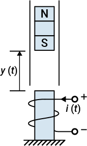
The equation of motion for this system is
where is the distance of the magnet above the electromagnet, is the current flowing in the electromagnet, is the mass of the magnet, and is the gravitational constant. The parameter is a viscous friction coefficient that is determined by the material in which the magnet moves, and is a field strength constant that is determined by the number of turns of wire on the electromagnet and the strength of the magnet.
The data set contains two time series, the current and the magnet position. Load the data set and extract the data from cell arrays.
[current,position] = maglev_dataset;
current = [current{:}]';
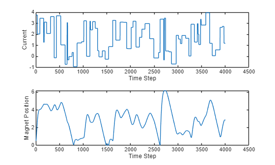
position = [position{:}]';Plot the data.
figure
tiledlayout(2,1)
nexttile
plot(current)
xlabel("Time Step")
ylabel("Current")
nexttile
plot(position)
xlabel("Time Step")
ylabel("Magnet Position")
Define NARX Network Architecture
NARX networks are a type of neural network architecture designed to handle nonlinear relationships in time series data. They are an extension of traditional autoregressive models by incorporating exogenous inputs, which are external factors that can influence the system. Mathematically, a NARX model can be expressed as
where is the output of the sequence at time step , is the exogenous input, and and are the number of delay steps considered for the sequence and the exogenous input respectively, i.e. the total number of past values considered in every prediction. When applied to the magnetic levitation system, the output corresponds to the position of the magnet, the exogenous input corresponds to the current.
In this example, you use a delay of two for the magnet position and the current. Therefore, the model becomes:
.
This diagram illustrates the architecture of a simple NARX network, showing the inputs and outputs for this problem.
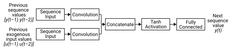
To create this NARX network, create a layer array containing a sequence input layer and a 1-D convolution layer. This layer array corresponds to the branch that receives the previous values in the sequence (the magnet position).
Set the size of the sequence input layer to the number of channels of the input data. Specify the size of the convolution filters as equal to the delay.
inputSizeSequence = 1;
numSequenceDelays = 2;
numFilters = 15;

sequenceLayers = [
    sequenceInputLayer(inputSizeSequence,Name="sequenceInput",MinLength=numSequenceDelays)
    convolution1dLayer(numSequenceDelays,numFilters,Name="conv1")];

NARXNet = dlnetwork;
NARXNet = addLayers(NARXNet,sequenceLayers);
Create a layer array containing a sequence input layer, a 1-D convolution layer, a concatenation layer, a tanh layer, and a fully connected layer. This layer array corresponds to the branch that receives the exogenous inputs (the current) and the final three layers.
Set the size of the sequence input layer to the number of channels of the input data. Specify the size of the convolution filters as equal to the delay.
inputSizeExogenous = 1;
numExogenousDelays = 2;
outputSize = 1;

exogenousLayers = [
    sequenceInputLayer(inputSizeExogenous,Name="exogenousInput",MinLength=numExogenousDelays)
    convolution1dLayer(numExogenousDelays,numFilters,Name="conv2")
    concatenationLayer(1,2,Name="cat")
    tanhLayer
    fullyConnectedLayer(outputSize)];
Add these layers to the network and connect the 1-D convolution layer to the second input of the concatenation layer.
NARXNet = addLayers(NARXNet,exogenousLayers);
NARXNet = connectLayers(NARXNet,"conv1","cat/in2");
Training a NARX network can result in better accuracy when the learnable parameters have data type double. Initialize the learnable parameters and convert them to double using the dlupdate function.
NARXNet = initialize(NARXNet);
NARXNet = dlupdate(@double,NARXNet);
Split Training, Validation and Test Data
Partition the data into training, validation, and test data sets. Use the first 60% of the data for training, the next 20% of the data for testing, and the last 20% of the data for validation.
trainSplit = 0.6;
testSplit = 0.2;
inputSeqLength = numel(current)
inputSeqLength =
4001
numTrain = floor(inputSeqLength * trainSplit)
numTrain =
2400
numTest = floor(inputSeqLength * testSplit)
numTest =
800
numVal = inputSeqLength - numTrain - numTest
numVal =
801
For the training data, the predictors positionTrain and currentTrain contain the 1st to 2399th data points of the magnet position and current respectively, while the targets TTrain contain the 3rd to 2400th data points of the magnet position.
numDelays = max(numExogenousDelays,numSequenceDelays);

positionTrain = position(1+numDelays-numSequenceDelays:numTrain-1);
currentTrain = current(1+numDelays-numExogenousDelays:numTrain-1);
TTrain = position(1+numDelays:numTrain);
When training neural networks, it often helps to make sure that your data is normalized in all stages of the network. Normalization helps stabilize and speed up network training using gradient descent.
Determine the mean and standard deviation of the position and current training data.
muPosition = mean(positionTrain);
sigmaPosition = std(positionTrain);
muCurrent = mean(currentTrain);
sigmaCurrent = std(currentTrain);
Normalize the training predictors and targets by subtracting the mean and scaling by the standard deviation.
currentTrain = (currentTrain - muCurrent) / sigmaCurrent;
positionTrain = (positionTrain - muPosition) / sigmaPosition;
TTrain = (TTrain - muPosition) / sigmaPosition;
To train a network with multiple inputs using the trainnet function, create a single datastore that contains the training predictors and targets. To convert numeric arrays to datastores, use arrayDatastore. Then, use the combine function to combine them into a single datastore.
NARXTrain = combine(arrayDatastore(positionTrain,IterationDimension=2),arrayDatastore(currentTrain,IterationDimension=2),arrayDatastore(TTrain,IterationDimension=2));
For the validation data predictions positionVal and currentVal, use the 3201st to 4000th data points of the magnet position and current respectively. For the validation targets TVal, use the 3203rd to 4001st data points of the magnet position.
positionVal = position(numTrain+numTest+1+numDelays-numSequenceDelays:end-1);
currentVal = current(numTrain+numTest+1+numDelays-numExogenousDelays:end-1);
TVal = position(numTrain+numTest+1+numDelays:end);
Normalize the validation predictors and targets by subtracting the mean and scaling by the standard deviation.
positionVal = (positionVal- muPosition) / sigmaPosition;
currentVal = (currentVal - muCurrent) / sigmaCurrent;
TVal = (TVal - muPosition) / sigmaPosition;
Create a single datastore that contains the validation predictors and targets.
NARXVal = combine(arrayDatastore(positionVal,IterationDimension=2),arrayDatastore(currentVal,IterationDimension=2),arrayDatastore(TVal,IterationDimension=2));
For the test data, the inputs positionTest and currentTest contain the 2401st to 3199th data points, while the targets TTest contain the 2403rd to 3200th data points.
positionTest = position(numTrain+1+numDelays-numSequenceDelays:numTrain+numTest-1);
currentTest = current(numTrain+1+numDelays-numExogenousDelays:numTrain+numTest-1);
TTest = position(numTrain+1+numDelays:numTrain+numTest);
Normalize the test predictors and targets by subtracting the mean and scaling by the standard deviation.
positionTest = (positionTest - muPosition) / sigmaPosition;
currentTest = (currentTest - muCurrent) / sigmaCurrent;
TTest = (TTest- muPosition) / sigmaPosition;
Create a single datastore that contains the test predictors and responses.
NARXTest = combine(arrayDatastore(positionTest,IterationDimension=2),arrayDatastore(currentTest,IterationDimension=2),arrayDatastore(TTest,IterationDimension=2));
Train Network
Specify the training options.
Use the Levenberg–Marquardt (LM) solver. LM is a suitable solver for small networks and data sets that can be processed in a single batch.
Plot the training progress and disable verbose output.
Specify the validation data.
Set the maximum number of iterations to 500 and the relative gradient tolerance and step size tolerance to to give the network sufficient time to train.
options = trainingOptions("lm", ...
    Plots="training-progress", ...
    Verbose=false, ...
    ValidationData=NARXVal, ...
    MaxIterations=500, ...
    GradientTolerance=1e-8, ...
    StepTolerance=1e-8);
Train the network using the trainnet function. By default, trainnet uses a GPU if one is available; otherwise, it uses a CPU. Training on a GPU requires Parallel Computing Toolbox™ and a supported GPU device. For information on supported devices, see GPU Computing Requirements (Parallel Computing Toolbox). You can also specify the execution environment by using the ExecutionEnvironment name-value argument of trainingOptions.
trainedNARXNet = trainnet(NARXTrain,NARXNet,"mse",options);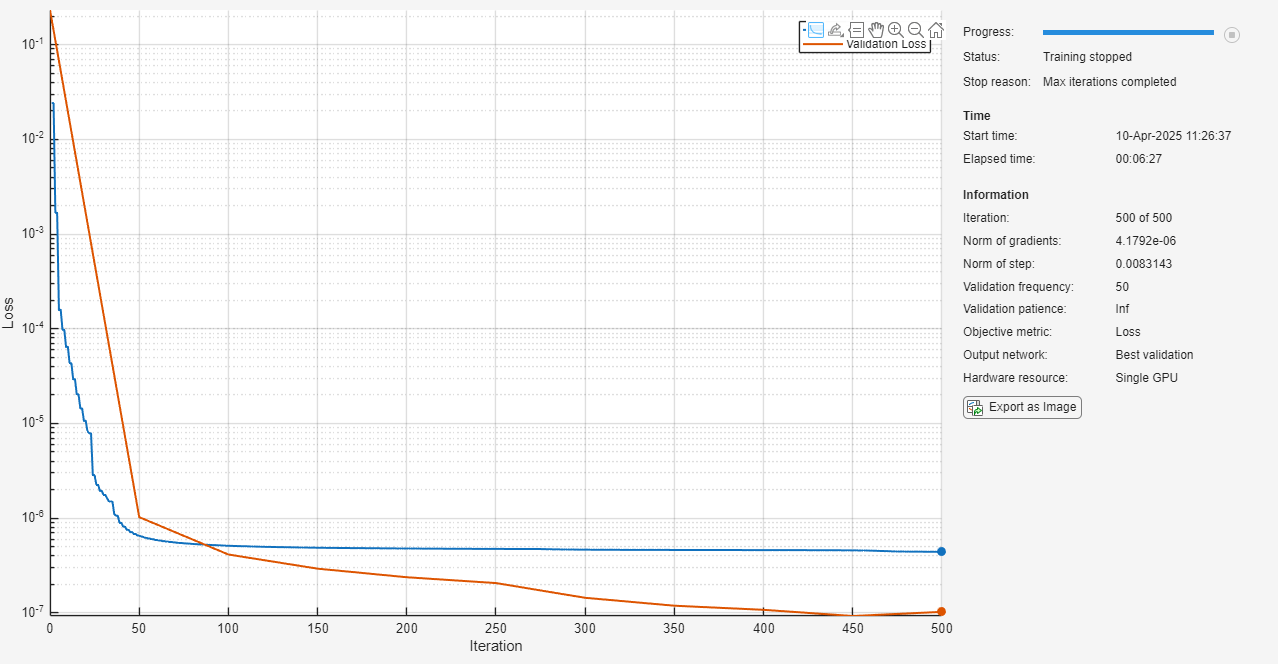
Test Network
Forecast the magnet position using the trained networks. In this example, both open-loop and closed-loop forecasting will be performed. Open-loop forecasting involves using actual observations as inputs to predict future values. Closed-loop forecasting, on the other hand, uses the model's own predictions as inputs for future forecasts.
Make open-loop predictions using the Make Predictions Using dlnetwork Object function and provide the entire test data set as input.
YNARXOpen = predict(trainedNARXNet,positionTest,currentTest);
To test the network's ability to make closed-loop predictions:
Create an array containing only the first two elements of the magnet position test data, and use that array to make an initial prediction.
Add the prediction to the end of the array of magnet positions.
Iteratively make further predictions using the last two elements of the array.
Remove the first two elements from the array.
YNARXClosed = positionTest(1:numSequenceDelays);

for idx = 1:numTest-numDelays
    YNARXClosed(end+1) = predict(trainedNARXNet,YNARXClosed(end-numSequenceDelays+1:end),currentTest(idx:idx+numExogenousDelays-1));
end
YNARXClosed = YNARXClosed(numDelays+1:end);
Compare the predictions to the targets.
positionTrainTest = (position(1:numTrain+numTest) - muPosition) / sigmaPosition;

figure
plot(positionTrainTest)
hold on
plot((1:numel(YNARXOpen))+numTrain+numDelays,YNARXOpen,"--")
plot((1:numel(YNARXClosed))+numTrain,YNARXClosed,"--")
xlabel("Time Step")
ylabel("Magnet Position (normalized)")
title("NARX Network Predictions")
legend("Targets","Open-Loop Predictions","Closed-Loop Predictions",Location="northwest")
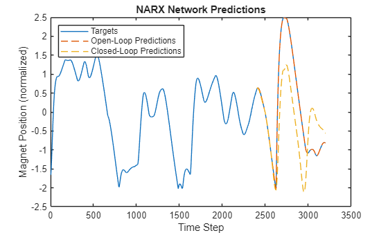
Calculate the root mean squared error (RMSE) of the predictions.
rmseNARXOpen = rmse(YNARXOpen,TTest)
rmseNARXOpen =
0.0046
rmseNARXClosed = rmse(YNARXClosed,TTest)
rmseNARXClosed =
0.9063
Save the trained network.
save("trainedNARXNet.mat","trainedNARXNet")
Export Network to Simulink
Export the trained neural network to Simulink using the exportNetworkToSimulink function. This function converts the network into layer blocks. You can use layer blocks to:
Visualize the operations of each layer in a network.
Easily debug issues with a Simulink model and generated code.
Customized generated code using built-in Simulink® features.
The exportNetworkToSimulink function creates a Simulink model, my_model, with two input ports, a Layer Blocks subsystem, and an output port. As the network makes predictions using several delayed versions of the input signals, specify that the exported network should use frame-based processing.
exportNetworkToSimulink(trainedNARXNet,FrameBased=true);
The subsystem my_model contains the neural network described using layer blocks. Click inside the subsystem to see the layer blocks. Each block represents a layer.
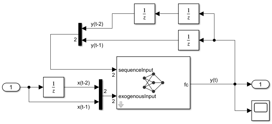
Integrate Network into Simulink Model
Open a Simulink model that takes the exogenous current signal as input, and uses delayed predictions as input to the network. The model uses Unit Delay (Simulink) blocks to delay both inputs to the network. This model has an empty placeholder NARX network subsystem.
mdl = "NARXNetModel";
open_system(mdl)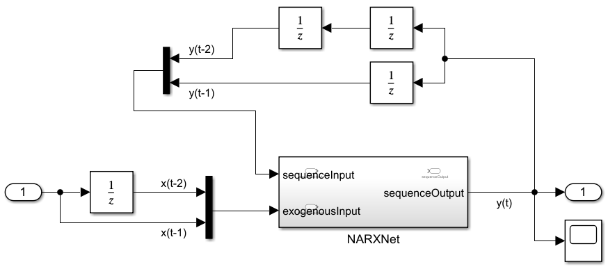
Copy the generated Layer Blocks subsystem, my_model, paste it inside the NARXNet subsystem, and connect the input and output ports.
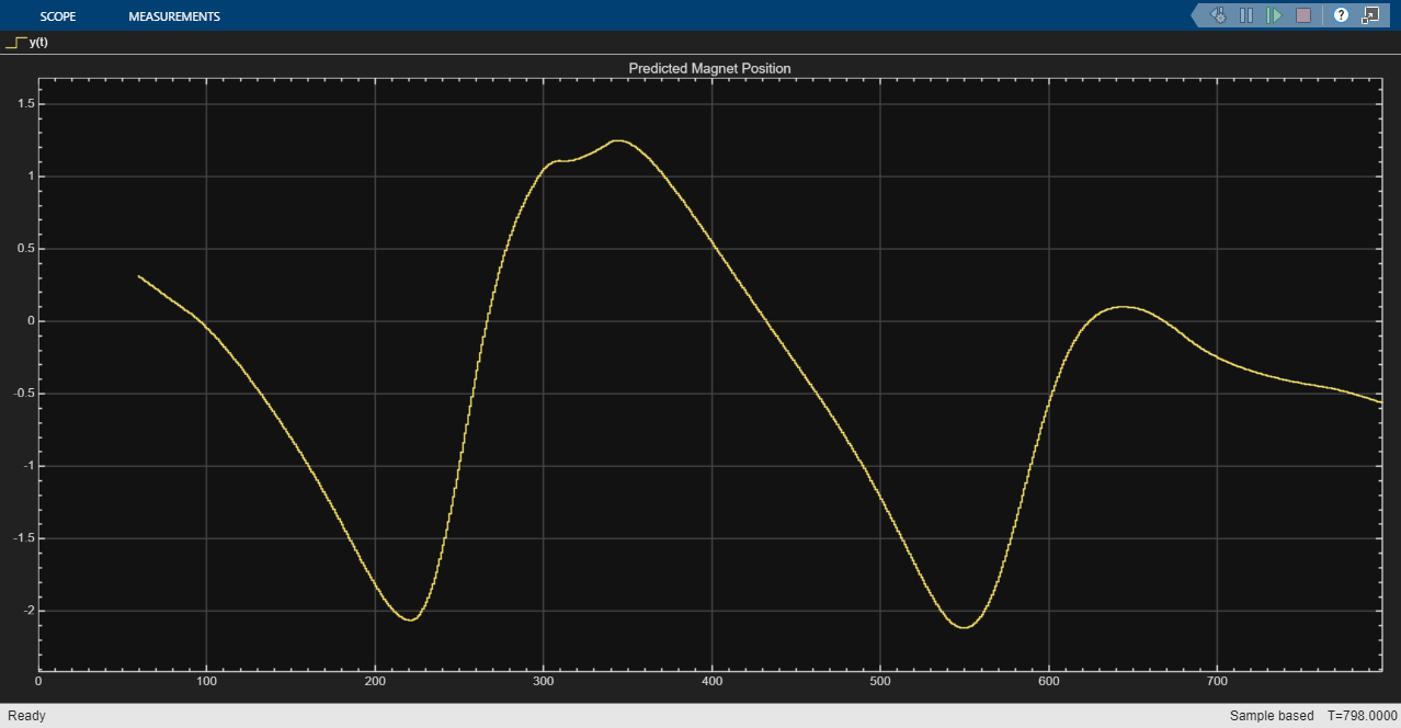
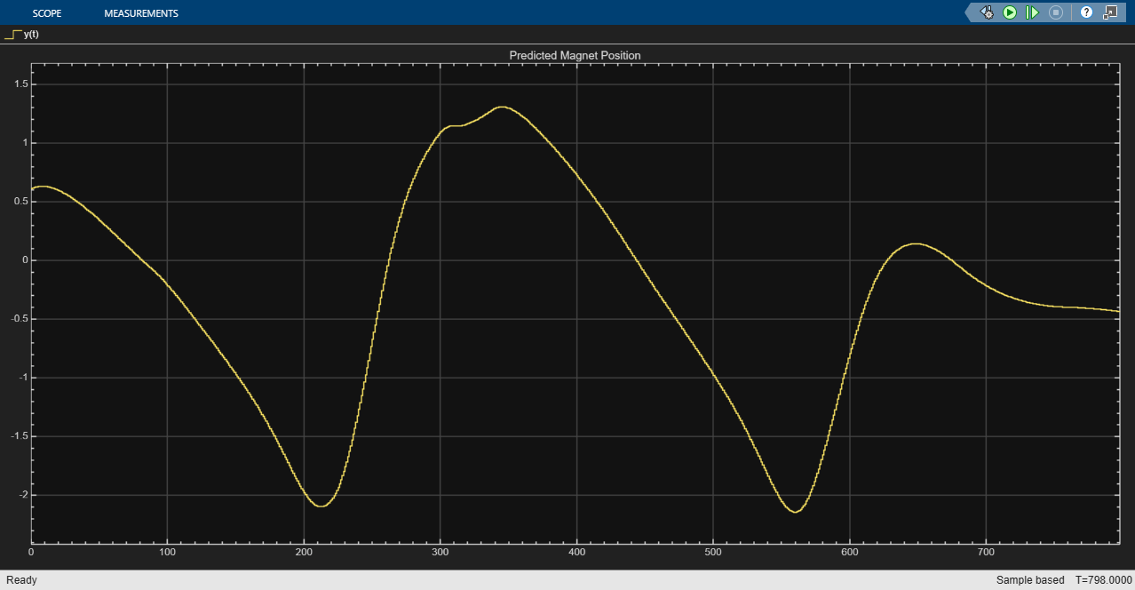
Simulate Using Test Data
Test the performance of the trained network in Simulink using the NARXNet model.
Set the initial condition of the Unit Delay blocks for the sequence input using the first two elements of the test position data.
set_param(mdl+"/Unit Delay","InitialCondition",string(positionTest(2)))
set_param(mdl+"/Unit Delay1","InitialCondition",string(positionTest(2)))
set_param(mdl+"/Unit Delay2","InitialCondition",string(positionTest(1)))
Set the initial condition of the Unit Delay block for the exogenous input using the element of the test current data.
set_param(mdl+"/Unit Delay3","InitialCondition",string(currentTest(1)))
Remove the first element from the test current data array (as it is already provided by the initial condition of the Unit Delay block) and create a corresponding vector of time steps. The model takes the variables X1NARXTest and t as input.
currentTest = currentTest(2:end);
t = (0:1:numel(currentTest)-1)';
Run the model.
simOut = sim(mdl);
Extract the results of the simulation. Discard the last element as there is no data in the test target data set to test its accuracy.
YNARXSimClosed = simOut.yout{1}.Values.Data(1:end-1);Calculate the RMSE of the predictions. The RMSE matches the RMSE of the closed-loop predictions made in MATLAB.
rmseNARXSimClosed = rmse(YNARXSimClosed,TTest)
rmseNARXSimClosed =
0.9063
See Also
trainnet | trainingOptions | dlnetwork | convolution1dLayer | sequenceInputLayer
Topics
- Compare Deep Learning and ARMA Models for Time Series Modeling
- Time Series Forecasting Using Deep Learning
- Sequence Classification Using Deep Learning
- Sequence-to-Sequence Classification Using Deep Learning
- Sequence-to-Sequence Regression Using Deep Learning
- Sequence-to-One Regression Using Deep Learning
- Long Short-Term Memory Neural Networks
- Deep Learning in MATLAB