portfolioCostCurves
Estimate market-impact cost of order execution for portfolio
Description
pcc = portfolioCostCurves(k,portfolio,tradeQuantity,tqRange,tradeStrategy,tsRange)
Kissell Research Group (KRG) transaction cost analysis object
kPortfolio data
portfolioTrade quantity
tradeQuantitywith a range of valuestqRangeTrade strategy
tradeStrategywith a range of valuestsRange
Examples
Retrieve the market impact data from the KRG FTP site. Connect to the FTP site using the
ftp function with a user name and password. Navigate to the
MI_Parameters folder and retrieve the market impact data in the
MI_Encrypted_Parameters.csv file. miData contains
the encrypted market impact date, code, and parameters.
f = ftp('ftp.kissellresearch.com','username','pwd');
mget(f,'MI_Encrypted_Parameters.csv');

miData = readtable('MI_Encrypted_Parameters.csv','delimiter', ...
    ',','ReadRowNames',false,'ReadVariableNames',true);
Create a Kissell Research Group transaction cost analysis object
k.
k = krg(miData);
Load the example portfolio data from the file
KRGExampleData.mat, which is included with the
Datafeed Toolbox™.
load KRGExampleDataThe variable PortfolioData appears in the MATLAB® workspace.
PortfolioData contains these variables:
Stock symbol
Local price
Price in a different currency if applicable
Average daily volume
Volatility
Number of shares
For a description of the example data, see Interpret Variables in Kissell Research Group Data Sets.
Estimate market-impact cost for an order execution on
a portfolio of assets. Specify the trade quantity as DollarValue.
Specify the trade quantity range tqRange with increments
of $10,000,000. Start with a total portfolio value of $100,000,000
and end with $500,000,000. Set the percentage of volume trading strategy POV.
Specify the trade strategy range tsRange with increments
of 10% by starting with a percentage of volume of 10% and ending with
40%.
tqRange = (100000000:10000000:500000000);
tsRange = (0.10:0.10:0.40);

pcc = portfolioCostCurves(k,PortfolioData,'DollarValue',tqRange,...
'POV',tsRange);
Display the first three rows of market-impact cost data.
pcc(1:3,:)
ans =

    Size      Shares       TradeValue     AbsTradeValue    POV     TradeTime    Cost_bp    Cost_DollarsPerShare    Cost_Dollars
    ____    __________    ____________    _____________    ____    _________    _______    ____________________    ____________

    0.02    5612057.03    100000000.00    328737579.09     0.10    0.18         38.74      0.07                    387447.95
    0.02    5612057.03    100000000.00    328737579.09     0.20    0.08         61.18      0.11                    611819.30
    0.02    5612057.03    100000000.00    328737579.09     0.30    0.05         80.07      0.14                    800683.38
The market-impact cost data contains:
Average trade size across all stocks in the portfolio
Number of shares in the transaction
Sum of traded value across all stocks in the portfolio
Sum of absolute value of the trade value across all stocks in the portfolio
Average execution percentage of volume to complete the number of shares
Average trade time in percentage of the day to complete the number of shares
Market-impact cost in basis points of local price
Market-impact cost in dollars per share
Market-impact cost in total dollar value
Display portfolio cost curves for percentage of volume rates: 10%, 20%, 30%, and 40%.
figure
size10 = pcc.Size(1:4:end)*100;
size20 = pcc.Size(2:4:end)*100;
size30 = pcc.Size(3:4:end)*100;
size40 = pcc.Size(4:4:end)*100;
cost10 = pcc.Cost_bp(1:4:end);
cost20 = pcc.Cost_bp(2:4:end);
cost30 = pcc.Cost_bp(3:4:end);
cost40 = pcc.Cost_bp(4:4:end);
plot(size10,cost10,size20,cost20,size30,cost30,size40,cost40)
grid on
axis([2 11 25 200])
xlabel({'Size','(%ADV)'})
ylabel({'Cost','(bps)'})
legend('POV = 10%','POV = 20%','POV = 30%','POV = 40%',...
'Location','northwest')
title('Portfolio Costs')
a = gca;
a.XAxis.TickLabelFormat = '%g%%';
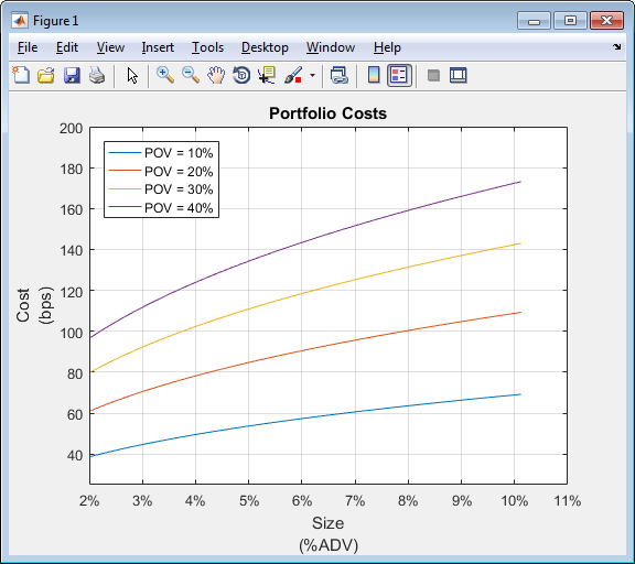
This figure demonstrates using portfolio costs to construct the portfolio and manage portfolio contents. By analyzing portfolio costs, you can determine the optimal portfolio size.
Input Arguments
Output Arguments
Tips
To test multiple portfolio transactions, you can use different ranges. You can change the percentage of shares in the transaction or use a different trade strategy. For details, see Input Arguments.
For details about the calculations, contact Kissell Research Group.
References
[1] Kissell, Robert. “A Practical Framework for Transaction Cost Analysis.” Journal of Trading. Vol. 3, Number 2, Summer 2008, pp. 29–37.
[2] Kissell, Robert. “Algorithmic Trading Strategies.” Ph.D. Thesis. Fordham University, May 2006.
[3] Kissell, Robert. “TCA in the Investment Process: An Overview.” Journal of Index Investing. Vol. 2, Number 1, Summer 2011, pp. 60–64.
[4] Kissell, Robert. The Science of Algorithmic Trading and Portfolio Management. Cambridge, MA: Elsevier/Academic Press, 2013.
[5] Kissell, Robert, and Morton Glantz. Optimal Trading Strategies. New York, NY: AMACOM, Inc., 2003.
Version History
Introduced in R2016a
See Also
krg | costCurves | iStar | marketImpact | timingRisk