Fit Exponential Model to Data

This example shows how to fit an exponential model to data using the trust-region and Levenberg-Marquardt nonlinear least-squares algorithms.

Load the census data set.

load census

The variables pop and cdate contain data for the population size and the year the census was taken, respectively.

Display a scatter plot of the data.

scatter(cdate,pop)
xlabel("Year")
ylabel("Population")

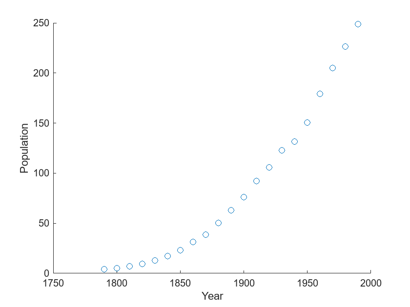
The plot shows that the population increases from year to year in a shape that resembles an exponential function.

Fit a two-term exponential model to the population data using the default trust-region fitting algorithm. Return the results of the fit and the goodness-of-fit statistics.

[exp_tr,gof_tr] = fit(cdate,pop,"exp2")

exp_tr = 
     General model Exp2:
     exp_tr(x) = a*exp(b*x) + c*exp(d*x)
     Coefficients (with 95% confidence bounds):
       a =   7.169e-17
       b =     0.02155
       c =           0
       d =     0.02155

gof_tr = struct with fields:
           sse: 1.2412e+04
       rsquare: 0.8995
           dfe: 17
    adjrsquare: 0.8818
          rmse: 27.0209

exp_tr contains the results of the fit, including coefficients calculated with the trust-region fitting algorithm. The goodness-of-fit statistics stored in gof_tr include the root mean squared error (RMSE) of 27.0209.

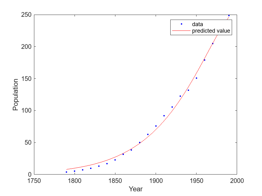
Plot the model in exp_tr together with a scatter plot of the data.

plot(exp_tr,cdate,pop)
legend(["data","predicted value"])
xlabel("Year")
ylabel("Population")

The plot shows that the model in exp_tr does not closely follow the census data.

Improve the fit by using the Levenberg-Marquardt fitting algorithm to calculate the coefficients.

[exp_lm,gof_lm] = fit(cdate,pop,"exp2",Algorithm="Levenberg-Marquardt")

exp_lm = 
     General model Exp2:
     exp_lm(x) = a*exp(b*x) + c*exp(d*x)
     Coefficients (with 95% confidence bounds):
       a =   4.282e-17  (-1.125e-11, 1.126e-11)
       b =     0.02477  (-5.67, 5.719)
       c =  -3.933e-17  (-1.126e-11, 1.126e-11)
       d =     0.02481  (-5.696, 5.745)

gof_lm = struct with fields:
           sse: 475.9498
       rsquare: 0.9961
           dfe: 17
    adjrsquare: 0.9955
          rmse: 5.2912

exp_lm contains the results of the fit, including coefficients calculated with the Levenberg-Marquardt fitting algorithm. The goodness-of-fit statistics stored in gof_lm include the RMSE of 5.2912, which is smaller than the RMSE for exp_tr. The relative sizes of the RMSEs indicate that the model stored in exp_lm fits the data more accurately than the model stored in exp_tr.

Plot the model in exp_lm together with a scatter plot of the data.

plot(exp_lm,cdate,pop)
legend(["data","predicted value"])
xlabel("Year")
ylabel("Population")

The plot shows that the model in exp_lm follows the census data more closely than the model in exp_tr.