Constructing and Working with B-form Splines
Construction of B-form
Usually, a spline is constructed from some information, like function values and/or
derivative values, or as the approximate solution of some ordinary differential
equation. But it is also possible to make up a spline from scratch, by providing its
knot sequence and its coefficient sequence to the command spmak.
For example, if you enter
sp = spmak(1:10,3:8);
you supply the uniform knot sequence 1:10 and the coefficient
sequence 3:8. Because there are 10 knots and 6 coefficients, the
order must be 4(= 10 – 6), i.e., you get a cubic spline. The command
fnbrk(sp)
prints out the constituent parts of the B-form of this cubic spline, as follows:
knots(1:n+k)
   1 2 3 4 5 6 7 8 9 10
coefficients(d,n)
   3 4 5 6 7 8
number n of coefficients
   6
order k
   4
dimension d of target
   1
Further, fnbrk can be used to supply each of these parts
separately.
But the point of the Curve Fitting Toolbox™ spline functionality is that there shouldn't be any need for you to look
up these details. You simply use sp as an argument to commands that
evaluate, differentiate, integrate, convert, or plot the spline whose description is
contained in sp.
Working With B-form Splines
The following commands are available for spline work. There is spmak and fnbrk to make up a spline and take it
apart again. Use fn2fm to convert from B-form to ppform.
You can evaluate, differentiate, integrate, minimize, find zeros of, plot, refine, or
selectively extrapolate a spline with the aid of fnval,
fnder, fndir, fnint,
fnmin, fnzeros, fnplt,
fnrfn, and fnxtr.
There are five commands for generating knot sequences:
augkntfor providing boundary knots and also controlling the multiplicity of interior knotsbrk2kntfor supplying a knot sequence with specified multiplicitiesaptkntfor providing a knot sequence for a spline space of given order that is suitable for interpolation at given data sitesoptkntfor providing an optimal knot sequence for interpolation at given sitesnewkntfor a knot sequence perhaps more suitable for the function to be approximated
In addition, there is:
To display a spline curve with given two-dimensional coefficient
sequence and a uniform knot sequence, use spcrv.
You can also write your own spline construction commands, in which case you will need
to know the following. The construction of a spline satisfying some interpolation or
approximation conditions usually requires a collocation matrix, i.e., the matrix that, in each row,
contains the sequence of numbers
DrBj,k(τ),
i.e., the rth derivative at τ of the jth B-spline,
for all j, for some r and some site τ. Such a
matrix is provided by spcol. An optional argument allows for this matrix to be
supplied by spcol in a space-saving spline-almost-block-diagonal-form
or as a MATLAB® sparse matrix. It can be fed to slvblk, a command for
solving linear systems with an almost-block-diagonal coefficient matrix. If you are
interested in seeing how spcol and slvblk are used
in this toolbox, have a look at the commands spapi,
spap2, and spaps.
In addition, there are routines for constructing cubic splines.
csapi and csape provide the cubic spline
interpolant at knots to given data, using the not-a-knot and various other end
conditions, respectively. A parametric cubic spline curve through given points is
provided by cscvn. The cubic smoothing spline is
constructed in csaps.
Example: B-form Spline Approximation to a Circle
As another simple example,
points = .95*[0 -1 0 1;1 0 -1 0];
sp = spmak(-4:8,[points points]);
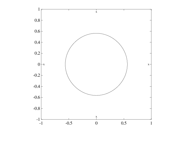
provides a planar, quartic, spline curve whose middle part is a pretty good approximation to a circle, as the plot on the next page shows. It is generated by a subsequent
plot(points(1,:),points(2,:),'x'), hold on
fnplt(sp,[0,4]), axis equal square, hold off
Insertion of additional control points would make a visually perfect circle.
Here are more details. The spline curve
generated has the form Σ8j=1Bj,5a(:, j),
with -4:8 the uniform knot sequence, and with its
control points a(:,j) the sequence (0,α),(–α,0),(0,–α),(α,0),(0,α),(–α,0),(0,–α),(α,0) with α=0.95.
Only the curve part between the parameter values 0 and 4 is actually
plotted.
To get a feeling for how close to circular this part of the curve actually is, compute its unsigned curvature. The curvature κ(t) at the curve point γ(t) = (x(t), y(t)) of a space curve γ can be computed from the formula
in which x', x″, y', and y” are the first and second derivatives of the curve with respect to the parameter used (t). Treat the planar curve as a space curve in the (x,y)-plane, hence obtain the maximum and minimum of its curvature at 21 points as follows:
t = linspace(0,4,21);zt = zeros(size(t));
dsp = fnder(sp); dspt = fnval(dsp,t); ddspt = fnval(fnder(dsp),t);
kappa = abs(dspt(1,:).*ddspt(2,:)-dspt(2,:).*ddspt(1,:))./...
   (sum(dspt.^2)).^(3/2);
[min(kappa),max(kappa)]

ans =
     1.6747    1.8611
So, while the curvature is not quite constant, it is close to 1/radius of the circle, as you see from the next calculation:
1/norm(fnval(sp,0))

ans =
     1.7864
Spline Approximation to a Circle; Control Points Are Marked
x
