Sparse Balanced Truncation of Thermal Model
Since R2023b
This example shows how to perform balanced truncation of a sparse state-space model obtained from linearizing a thermal model of heat distribution in a circular cylindrical rod.
Load the model data.
load cylindricalRod.mat
sys = sparss(A,B,C,D,E);
size(sys)
Sparse state-space model with 3 outputs, 1 inputs, and 7522 states.
The thermal model contains 7522 states.
Create a balanced truncation specification object for sys and run the algorithm.
R = reducespec(sys,"balanced");
R = process(R)
Initializing... Running ADI with built-in shifts......... Solved Lyapunov equations to desired accuracy.
R =
  SparseBalancedTruncation with properties:

        Sigma: [36×1 double]
       Energy: [36×1 double]
        Error: [36×1 double]
           Lr: [7522×36 double]
           Lo: [7522×123 double]
    Residuals: [6.1259e-09 1.6131e-09]
      Options: [1×1 mor.SparseBalancedTruncationOptions]
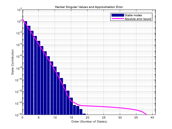
Use the view command to visualize the state contributions as Hankel singular values.
view(R,"sigma")Obtain the reduced-order model with maximum error of 1e-6. This results in a model with order 8.
rsys = getrom(R,MaxError=1e-6,Method="truncate");Compare the singular value response of the models.
w = logspace(-7,-3,20);
fsys = frd(sys,w);
sigma(fsys,fsys-rsys,'r--')

The reduced-order model is a good match for the full-order model.
See Also
Functions
Objects
Topics
- Task-Based Model Order Reduction Workflow
- Sparse Model Basics
- Heat Distribution in Circular Cylindrical Rod (Partial Differential Equation Toolbox)