Active Vibration Control in Three-Story Building

This example uses systune to control seismic vibrations in a three-story building.

Background

This example considers an Active Mass Driver (AMD) control system for vibration isolation in a three-story experimental structure. This setup is used to assess control design techniques for increasing safety of civil engineering structures during earthquakes. The structure consists of three stories with an active mass driver on the top floor which is used to attenuate ground disturbances. This application is borrowed from "Benchmark Problems in Structural Control: Part I - Active Mass Driver System," B.F. Spencer Jr., S.J. Dyke, and H.S. Deoskar, Earthquake Engineering and Structural Dynamics, 27(11), 1998, pp. 1127-1139.

Figure 1: Active Mass Driver Control System

The plant P is a 28-state model with the following state variables:

• x(i): displacement of i-th floor relative to the ground (cm)

• xm: displacement of AMD relative to 3rd floor (cm)

• xv(i): velocity of i-th floor relative to the ground (cm/s)

• xvm: velocity of AMD relative to the ground (cm/s)

• xa(i): acceleration of i-th floor relative to the ground (g)

• xam: acceleration of AMD relative to the ground (g)

• d(1)=x(1), d(2)=x(2)-x(1), d(3)=x(3)-x(2): inter-story drifts

The inputs are the ground acceleration xag (in g) and the control signal u. We use 1 g = 981 cm/s^2.

load ThreeStoryData
size(P)

State-space model with 20 outputs, 2 inputs, and 28 states.

Model of Earthquake Acceleration

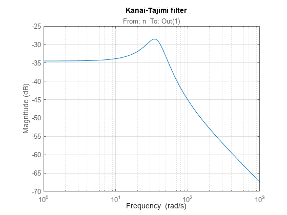
The earthquake acceleration is modeled as a white noise process filtered through a Kanai-Tajimi filter.

zg = 0.3;
wg = 37.3; 
S0 = 0.03*zg/(pi*wg*(4*zg^2+1));
Numerator = sqrt(S0)*[2*zg*wg wg^2];
Denominator = [1 2*zg*wg wg^2];

F = sqrt(2*pi)*tf(Numerator,Denominator);
F.InputName = 'n';   % white noise input

bodemag(F)
grid
title('Kanai-Tajimi filter')

Open-Loop Characteristics

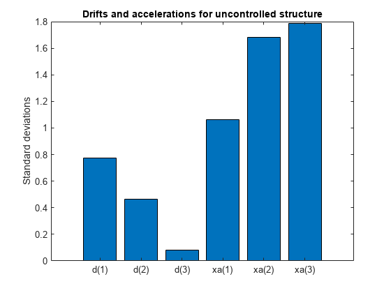
The effect of an earthquake on the uncontrolled structure can be simulated by injecting a white noise input n into the plant-filter combination. You can also use covar to directly compute the standard deviations of the resulting inter-story drifts and accelerations.

% Add Kanai-Tajimi filter to the plant
PF = P*append(F,1); 

% Standard deviations of open-loop drifts
CV = covar(PF('d','n'),1);
d0 = sqrt(diag(CV));

% Standard deviations of open-loop acceleration 
CV = covar(PF('xa','n'),1);
xa0 = sqrt(diag(CV));

% Plot open-loop RMS values 
clf
bar([d0; xa0])
title('Drifts and accelerations for uncontrolled structure')
ylabel('Standard deviations')
set(gca,'XTickLabel',{'d(1)','d(2)','d(3)','xa(1)','xa(2)','xa(3)'})

Control Structure and Design Requirements

The control structure is depicted in Figure 2.

Figure 2: Control Structure

The controller $$C$$ uses measurements yxa and yxam of xa and xam to generate the control signal u. Physically, the control u is an electrical current driving an hydraulic actuator that moves the masses of the AMD. The design requirements involve:

• Minimization of the inter-story drifts d(i) and accelerations xa(i)

• Hard constraints on control effort in terms of mass displacement xm, mass acceleration xam, and control effort u

All design requirements are assessed in terms of standard deviations of the corresponding signals. Use TuningGoal.Variance to express these requirements and scale each variable by its open-loop standard deviation to seek uniform relative improvement in all variables.

% Soft requirements on drifts and accelerations 
Soft = [...
   TuningGoal.Variance('n','d(1)',d0(1)) ; ...
   TuningGoal.Variance('n','d(2)',d0(2)) ; ...
   TuningGoal.Variance('n','d(3)',d0(3)) ; ...
   TuningGoal.Variance('n','xa(1)',xa0(1)) ; ...
   TuningGoal.Variance('n','xa(2)',xa0(2)) ; ...
   TuningGoal.Variance('n','xa(3)',xa0(3))];

% Hard requirements on control effort
Hard = [...
   TuningGoal.Variance('n','xm',3) ; ...
   TuningGoal.Variance('n','xam',2) ; ...
   TuningGoal.Variance('n','u',1)];

Controller Tuning

systune lets you tune virtually any controller structure subject to these requirements. The controller complexity can be adjusted by trial-and-error, starting with sufficiently high order to gauge the limits of performance, then reducing the order until you observe a noticeable performance degradation. For this example, start with a 5th-order controller with no feedthrough term.

C = tunableSS('C',5,1,4);
C.D.Value = 0;
C.D.Free = false;   % Fix feedthrough to zero

Construct a tunable model T0 of the closed-loop system of Figure 2 and tune the controller parameters with systune.

% Build tunable closed-loop model 
T0 = lft(PF,C); 

% Tune controller parameters
[T,fSoft,gHard]  = systune(T0,Soft,Hard);

Final: Soft = 0.601, Hard = 0.99851, Iterations = 201

The summary indicates that we achieved an overall reduction of 40% in standard deviations (Soft = 0.6) while meeting all hard constraints (Hard < 1).

Validation

Compute the standard deviations of the drifts and accelerations for the controlled structure and compare with the uncontrolled results. The AMD control system yields significant reduction of both drift and acceleration.

% Standard deviations of closed-loop drifts
CV = covar(T('d','n'),1);
d = sqrt(diag(CV));

% Standard deviations of closed-loop acceleration 
CV = covar(T('xa','n'),1);
xa = sqrt(diag(CV));

% Compare open- and closed-loop values
clf
bar([d0 d; xa0 xa])
title('Drifts and accelerations')
ylabel('Standard deviations')
set(gca,'XTickLabel',{'d(1)','d(2)','d(3)','xa(1)','xa(2)','xa(3)'})
legend('Uncontrolled','Controlled','location','NorthWest')

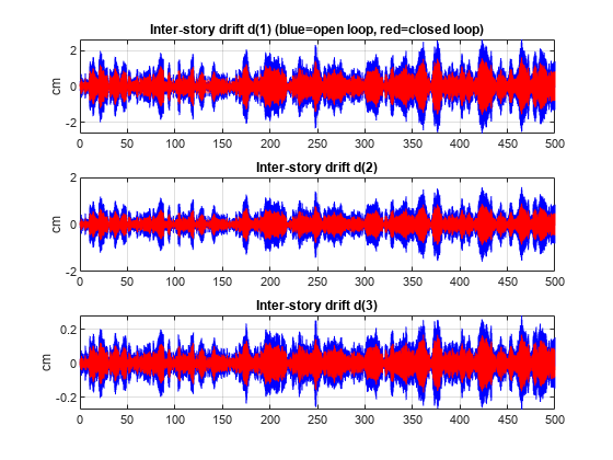
Simulate the response of the 3-story structure to an earthquake-like excitation in both open and closed loop. The earthquake acceleration is modeled as a white noise process colored by the Kanai-Tajimi filter.

% Sampled white noise process
rng('default')
dt = 1e-3; 
t = 0:dt:500;
n = randn(1,length(t))/sqrt(dt); % white noise signal

% Open-loop simulation
ysimOL = lsim(PF(:,1), n , t); 

% Closed-loop simulation 
ysimCL = lsim(T, n , t); 

% Drifts
clf
subplot(3,1,1) 
plot(t,ysimOL(:,13),'b',t,ysimCL(:,13),'r')
grid
title('Inter-story drift d(1) (blue=open loop, red=closed loop)')
ylabel('cm')
subplot(3,1,2)
plot(t,ysimOL(:,14),'b',t,ysimCL(:,14),'r')
grid 
title('Inter-story drift d(2)')
ylabel('cm')
subplot(3,1,3)
plot(t,ysimOL(:,15),'b',t,ysimCL(:,15),'r')
grid 
title('Inter-story drift d(3)')
ylabel('cm')

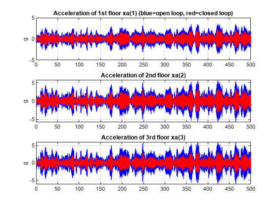
Accelerations

clf
subplot(3,1,1)
plot(t,ysimOL(:,9),'b',t,ysimCL(:,9),'r')
grid
title('Acceleration of 1st floor xa(1) (blue=open loop, red=closed loop)')
ylabel('g')
subplot(3,1,2)
plot(t,ysimOL(:,10),'b',t,ysimCL(:,10),'r')
grid
title('Acceleration of 2nd floor xa(2)')
ylabel('g')
subplot(3,1,3)
plot(t,ysimOL(:,11),'b',t,ysimCL(:,11),'r')
grid
title('Acceleration of 3rd floor xa(3)')
ylabel('g')

Control variables

clf
subplot(3,1,1)
plot(t,ysimCL(:,4),'r')
grid 
title('AMD position xm')
ylabel('cm') 
subplot(3,1,2)
plot(t,ysimCL(:,12),'r')
grid 
title('AMD acceleration xam')
ylabel('g') 
subplot(3,1,3)
plot(t,ysimCL(:,16),'r')
grid 
title('Control signal u')

Plot the root-mean-square (RMS) of the simulated signals for both the controlled and uncontrolled scenarios. Assuming ergodicity, the RMS performance can be estimated from a single sufficiently long simulation of the process and coincides with the standard deviations computed earlier. Indeed the RMS plot closely matches the standard deviation plot obtained earlier.

clf
bar([std(ysimOL(:,13:15)) std(ysimOL(:,9:11)) ; ...
   std(ysimCL(:,13:15)) std(ysimCL(:,9:11))]')
title('Drifts and accelerations')
ylabel('Simulated RMS values')
set(gca,'XTickLabel',{'d(1)','d(2)','d(3)','xa(1)','xa(2)','xa(3)'})
legend('Uncontrolled','Controlled','location','NorthWest')

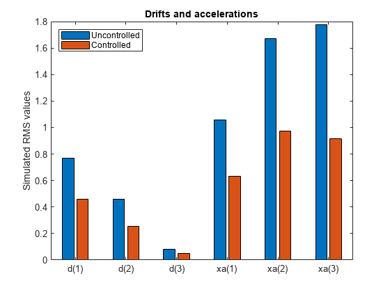
Overall, the controller achieves significant reduction of ground vibration both in terms of drift and acceleration for all stories while meeting the hard constraints on control effort and mass displacement.