Main Content

systune

Tune fixed-structure control systems modeled in MATLAB

Description

systune tunes fixed-structure control systems subject to both soft and hard design goals. systune can tune multiple fixed-order, fixed-structure control elements distributed over one or more feedback loops. For an overview of the tuning workflow, see Automated Tuning Workflow.

This command tunes control systems modeled in MATLAB®. For tuning Simulink® models, use slTuner (Simulink Control Design) to create an interface to your Simulink model. You can then tune the control system with systune (Simulink Control Design) for slTuner.

example

[CL,fSoft] = systune(CL0,SoftReqs) tunes the free parameters of the control system model, CL0, to best meet the soft tuning requirements. The best achieved soft constraint values are returned as fSoft. For robust tuning against real parameter uncertainty, use a control system model with uncertain real parameters. For robust tuning against a set of plant models, use an array of control system models CL0. (See Input Arguments.)

example

[CL,fSoft,gHard] = systune(CL0,SoftReqs,HardReqs) tunes the control system to best meet the soft tuning requirements subject to satisfying the hard tuning requirements (constraints). It returns the best achieved values for the soft and hard constraints.

[CL,fSoft,gHard] = systune(CL0,SoftReqs,HardReqs,options) specifies options for the optimization.

[CL,fSoft,gHard,info] = systune(___) also returns detailed information about each optimization run. All input arguments described for the previous syntaxes also apply here.

Examples

collapse all

Tune a cascaded control system to meet requirements of reference tracking and disturbance rejection.

The cascaded control system of the following illustration includes two tunable controllers, the PI controller for the inner loop, C2, and the PID controller for the outer loop, C1.

The blocks x1 and x2 mark analysis-point locations. These are locations at which loops can be opened or signals injected for the purpose of specifying requirements for tuning the system.

Tune the free parameters of this control system to meet the following requirements:

  • The output signal, y1, tracks the reference signal, r, with a response time of 10 seconds and a steady-state error of 1%.

  • A disturbance injected at x2 is suppressed at y1 by a factor of 10.

Create tunable Control Design Blocks to represent the controllers, and numeric LTI models to represent the plants. Also, create AnalysisPoint blocks to mark the points of interest in each feedback loop.

G2 = zpk([],-2,3);
G1 = zpk([],[-1 -1 -1],10);

C20 = tunablePID('C2','pi');
C10 = tunablePID('C1','pid');

X1 = AnalysisPoint('X1');
X2 = AnalysisPoint('X2');

Connect these components to build a model of the entire closed-loop control system.

InnerLoop = feedback(X2*G2*C20,1);
CL0 = feedback(G1*InnerLoop*C10,X1);
CL0.InputName = 'r';
CL0.OutputName = 'y';

CL0 is a tunable genss model. Specifying names for the input and output channels allows you to identify them when you specify tuning requirements for the system.

Specify tuning requirements for reference tracking and disturbance rejection.

Rtrack = TuningGoal.Tracking('r','y',10,0.01);
Rreject = TuningGoal.Gain('X2','y',0.1);

The TuningGoal.Tracking requirement specifies that the signal at 'y' track the signal at 'r' with a response time of 10 seconds and a tracking error of 1%.

The TuningGoal.Gain requirement limits the gain from the implicit input associated with the AnalysisPoint block, X2, to 'y'. (See AnalysisPoint.) Limiting this gain to a value less than 1 ensures that a disturbance injected at X2 is suppressed at the output.

Tune the control system.

[CL,fSoft] = systune(CL0,[Rtrack,Rreject]);
Final: Soft = 1.24, Hard = -Inf, Iterations = 107

systune converts each tuning requirement into a normalized scalar value, f. The command adjusts the tunable parameters of CL0 to minimize the f values. For each requirement, the requirement is satisfied if f < 1 and violated if f >1. fSoft is the vector of minimized f values. The largest of the minimized f values is displayed as Soft.

The output model CL is the tuned version of CL0. CL contains the same Control Design Blocks as CL0, with current values equal to the tuned parameter values.

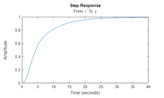
Validate that the tuned control system meets the tracking requirement by examining the step response from 'r' to 'y'.

stepplot(CL)

The step plot shows that in the tuned control system, CL, the output tracks the input with approximately the desired response time.

Validate the tuned system against the disturbance rejection requirement by examining the closed-loop response to a signal injected at X2.

CLdist = getIOTransfer(CL,'X2','y');
stepplot(CLdist);

getIOTransfer extracts the closed-loop response from the specified inputs to outputs. In general, getIOTransfer and getLoopTransfer are useful for validating a control system tuned with systune.

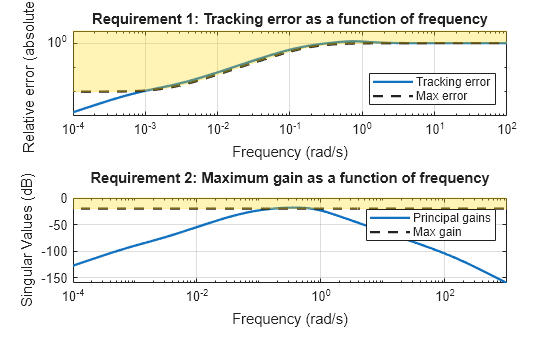
You can also use viewGoal to compare the responses of the tuned control system directly against the tuning requirements, Rtrack and Rreject.

viewGoal([Rtrack,Rreject],CL)

Tune a cascaded control system to meet requirements of reference tracking and disturbance rejection. These requirements are subject to a hard constraint on the stability margins of the inner and outer loops.

The cascaded control system of the following illustration includes two tunable controllers, the PI controller for the inner loop, C2, and the PID controller for the outer loop, C1.

The blocks x1 and x2 mark analysis-point locations. These are locations at which you can open loops or inject signals for the purpose of specifying requirements for tuning the system.

Tune the free parameters of this control system to meet the following requirements:

  • The output signal, y1, tracks the reference signal at r with a response time of 5 seconds and a steady-state error of 1%.

  • A disturbance injected at x2 is suppressed at the output, y1, by a factor of 10.

Impose these tuning requirements subject to hard constraints on the stability margins of both loops.

Create tunable Control Design Blocks to represent the controllers and numeric LTI models to represent the plants. Also, create AnalysisPoint blocks to mark the points of interest in each feedback loop.

G2 = zpk([],-2,3);
G1 = zpk([],[-1 -1 -1],10);

C20 = tunablePID('C2','pi');
C10 = tunablePID('C1','pid');

X1 = AnalysisPoint('X1');
X2 = AnalysisPoint('X2');

Connect these components to build a model of the entire closed-loop control system.

InnerLoop = feedback(X2*G2*C20,1);
CL0 = feedback(G1*InnerLoop*C10,X1);
CL0.InputName = 'r';
CL0.OutputName = 'y';

CL0 is a tunable genss model. Specifying names for the input and output channels allows you to identify them when you specify tuning requirements for the system.

Specify tuning requirements for reference tracking and disturbance rejection.

Rtrack = TuningGoal.Tracking('r','y',5,0.01);
Rreject = TuningGoal.Gain('X2','y',0.1);

The TuningGoal.Tracking requirement specifies that the signal at 'y' tracks the signal at 'r' with a response time of 5 seconds and a tracking error of 1%.

The TuningGoal.Gain requirement limits the gain from the implicit input associated with the AnalysisPoint block X2 to the output, 'y'. (See AnalysisPoint.) Limiting this gain to a value less than 1 ensures that a disturbance injected at X2 is suppressed at the output.

Specify tuning requirements for the gain and phase margins.

RmargOut = TuningGoal.Margins('X1',18,60);
RmargIn = TuningGoal.Margins('X2',18,60);
RmargIn.Openings = 'X1';

RmargOut imposes a minimum gain margin of 18 dB and a minimum phase margin of 60 degrees. Specifying X1 imposes that requirement on the outer loop. Similarly, RmargIn imposes the same requirements on the inner loop, identified by X2. To ensure that the inner-loop margins are evaluated with the outer loop open, include the outer-loop analysis-point location, X1, in RmargIn.Openings.

Tune the control system to meet the soft requirements of tracking and disturbance rejection, subject to the hard constraints of the stability margins.

SoftReqs = [Rtrack,Rreject];
HardReqs = [RmargIn,RmargOut];
[CL,fSoft,gHard] = systune(CL0,SoftReqs,HardReqs);
Final: Soft = 1.13, Hard = 0.97699, Iterations = 114

systune converts each tuning requirement into a normalized scalar value, f for the soft constraints and g for the hard constraints. The command adjusts the tunable parameters of CL0 to minimize the f values, subject to the constraint that each g < 1.

The displayed value Hard is the largest of the minimized g values in gHard. This value is less than 1, indicating that both the hard constraints are satisfied.

Validate the tuned control system against the stability margin requirements.

figure;
viewGoal(HardReqs,CL)

The viewGoal plot confirms that the stability margin requirements for both loops are satisfied by the tuned control system at all frequencies. The blue lines show the margin used in the optimization calculation, which is an upper bound on the actual margin of the tuned control system.

Examine whether the tuned control system meets the tracking requirement by examining the step response from 'r' to 'y'.

figure;
stepplot(CL,20)

The step plot shows that in the tuned control system, CL, the output tracks the input but the response is somewhat slower than desired and the tracking error may be larger than desired. For further information, examine the tracking requirement directly with viewGoal.

figure;
viewGoal(Rtrack,CL)

The actual tracking error crosses into the shaded area between 1 and 10 rad/s, indicating that the requirement is not met in this regime. Thus, the tuned control system cannot meet the soft tracking requirement, time subject to the hard constraints of the stability margins. To achieve the desired performance, you may need to relax one of your requirements or convert one or more hard constraints to soft constraints.

Input Arguments

collapse all

Control system to tune, specified as a generalized state-space (genss) model or array of models with tunable parameters. To construct CL0:

  1. Parameterize the tunable elements of your control system. You can use predefined structures, such as tunablePID, tunableGain, and tunableTF. Alternatively, you can create your own structure from elementary tunable parameters (realp).

  2. Build a closed-loop model of the overall control system as an interconnection of fixed and tunable components. To do so, use model interconnection commands such as feedback and connect. Use AnalysisPoint blocks to mark additional signals of interest for specifying and assessing tuning requirements.

For more information about creating models to tune, see Setup for Tuning Control System Modeled in MATLAB.

For robust tuning of a control system against a set of plant models (requires Robust Control Toolbox™), specify an array of tunable genss models that have the same tunable parameters. To make the controller robust against parameter uncertainty, use a model with uncertain real parameters defined with ureal (Robust Control Toolbox) or uss (Robust Control Toolbox). In this case, CL0 is a genss model that contains both tunable and uncertain control design blocks. For more information about robust tuning, see Robust Tuning Approaches (Robust Control Toolbox).

Soft tuning goals (objectives) for tuning the control system, specified as a vector of TuningGoal objects. These objects capture your design requirements, such as TuningGoal.Tracking, TuningGoal.StepTracking, or TuningGoal.Margins.

systune tunes the tunable parameters of the control system to minimize the soft tuning goals. This tuning is subject to satisfying the hard tuning goals (if any).

For more information about available tuning goals, see Tuning Goals.

Hard tuning goals (constraints) for tuning the control system, specified as a vector of TuningGoal objects. These objects capture your design requirements, such as TuningGoal.Tracking, TuningGoal.StepTracking, or TuningGoal.Margins.

systune converts each hard tuning goal to a normalized scalar value. systune then optimizes the free parameters to minimize those normalized values. A hard goal is satisfied if the normalized value is less than 1.

For more information about available tuning goals, see Tuning Goals.

Options for the tuning algorithm, specified as an options set you create with systuneOptions. Available options include:

  • Number of additional optimizations to run. Each optimization starts from random initial values of the free parameters.

  • Tolerance for terminating the optimization.

  • Flag for using parallel processing.

See the systuneOptions reference page for more details about all available options.

Output Arguments

collapse all

Tuned control system, returned as a generalized state-space (genss) model. This model has the same number and type of tunable elements (Control Design Blocks) as CL0. The current values of these elements are the tuned parameters. Use getBlockValue or showTunable to access values of the tuned elements.

If you provide an array of control system models to tune as the input argument, CL0, systune tunes the parameters of all the models simultaneously. In this case, CL is an array of tuned genss models. For more information, see Robust Tuning Approaches (Robust Control Toolbox).

Best achieved soft constraint values, returned as a vector. systune converts the soft requirements to a function of the free parameters of the control system. The command then tunes the parameters to minimize that function subject to the hard constraints. (See Algorithms.) fSoft contains the best achieved value for each of the soft constraints. These values appear in fSoft in the same order that the constraints are specified in SoftReqs. fSoft values are meaningful only when the hard constraints are satisfied.

Best achieved hard constraint values, returned as a vector. systune converts the hard requirements to a function of the free parameters of the control system. The command then tunes the parameters to drive those values below 1. (See Algorithms.) gHard contains the best achieved value for each of the hard constraints. These values appear in gHard in the same order that the constraints are specified in HardReqs. If all values are less than 1, then the hard constraints are satisfied.

Detailed information about each optimization run, returned as a data structure. The fields of info are summarized in the following table.

FieldValue
Run

Run number, returned as a scalar. If you use the RandomStart option of systuneOptions to perform multiple optimization runs, info is a structure array, and info.Run is the index.

Iterations

Total number of iterations performed during the run, returned as a scalar. If you use RandomStart, info.Iterations(j) is the number of iterations performed in the jth run before termination.

f

Best overall soft constraint value, returned as a scalar. systune converts the soft tuning goals to a function of the free parameters of the control system. The command then tunes the parameters to minimize that function subject to the hard goals. (See Algorithms.) info.f is the maximum soft goal value at the final iteration. This value is meaningful only when the hard goals are satisfied. If the value is less than 1, then the soft goals are also attained.

g

Best overall hard constraint value, returned as a scalar. systune converts the hard tuning goals to a function of the free parameters of the control system. The command then tunes the parameters to drive those values below 1. (See Algorithms.) info.g is the largest hard goal value at the final iteration. If this value is less than 1, then the hard goals are satisfied.

x

Tuned parameter values, returned as a vector. This vector contains the values of the tunable parameters at the end of the run. info.x can also include the values of additional variables such as loop scalings, if systune uses them (see info.LoopScaling).

MinDecay

Minimum decay rate of tuned system dynamics, returned as a two-element row vector.

info.MinDecay(1) is the minimum decay rate of the closed-loop poles.

info.MinDecay(2) is the minimum decay rate of the dynamics of tuned blocks with stability constraints. For more information about stabilized dynamics and decay rates, see the MinDecay option of systuneOptions.

fSoft

Individual soft constraint values, returned as a vector. systune converts each soft tuning goal to a normalized value that is a function of the free parameters of the control system. The command then tunes the parameters to minimize that value subject to the hard goals. (See Algorithms.) info.fSoft contains the individual values of the soft goals at the end of each run. These values appear in fSoft in the same order in which you specify goals in the SoftReqs input argument to systune.

gHard

Individual hard constraint values, returned as a vector. systune converts each hard tuning goal to a normalized value that is a function of the free parameters of the control system. The command then tunes the parameters to minimize those values. A hard goal is satisfied if its value is less than 1. (See Algorithms.) info.gHard contains the individual values of the hard goals at the end of each run. These values appear in gHard in the same order in which you specify goals in the HardReqs input argument to systune.

Blocks

Tuned values of tunable blocks and parameters in the tuned control system, returned as a structure whose fields are the names of tunable elements and whose values are the corresponding tuned values.

When you perform multiple runs by setting the RandomStart option to a positive value, you can use this field to examine control system performance with the results from other runs. For instance, use the following code to apply the tuned values from the jth run.

CLj = setBlockValue(CL0,info(j).Blocks)

LoopScaling

Optimal diagonal scaling for evaluating MIMO tuning requirements, returned as a state-space model.

When applied to multiloop control systems, tuning goals that involve an open-loop response can be sensitive to the scaling of the loop transfer functions to which they apply. This sensitivity can lead to poor optimization results. systune automatically corrects scaling issues and returns the optimal diagonal scaling matrix D as a state-space model in info.LoopScaling.

The loop channels associated with each diagonal entry of D are listed in info.LoopScaling.InputName. The scaled loop transfer is D\L*D, where L is the open-loop transfer measured at the locations info.LoopScaling.InputName.

Tuning goals affected by such loop scaling include:

  • TuningGoal.LoopShape

  • TuningGoal.MinLoopGain and TuningGoal.MaxLoopGain

  • TuningGoal.Sensitivity

  • TuningGoal.Rejection

  • TuningGoal.Margins

info also contains the following fields, whose entries are meaningful when you use systune for robust tuning of control systems with uncertainty.

FieldValue
wcPert

Worst combinations of uncertain parameters, returned as a structure array. Each structure contains one set of uncertain parameter values. The perturbations with the worst performance are listed first.

wcf

Worst soft-goal value, returned as a scalar. This value is the largest soft goal value (f) over the uncertainty range when using the tuned controller.

wcg

Worst hard-goal value, returned as a scalar. This value is the largest hard goal value (g) over the uncertainty range when using the tuned controller.

wcDecay

Smallest closed-loop decay rate over the uncertainty range when using the tuned controller, returned as a scalar. A positive value indicates robust stability. For more information about stabilized dynamics and decay rates, see the MinDecay option of systuneOptions.

Algorithms

x is the vector of tunable parameters in the control system to tune. systune converts each soft and hard tuning requirement SoftReqs(i) and HardReqs(j) into normalized values fi(x) and gj(x), respectively. systune then solves the constrained minimization problem:

Minimize maxifi(x) subject to maxjgj(x)<1, for xmin<x<xmax.

xmin and xmax are the minimum and maximum values of the free parameters of the control system.

When you use both soft and hard tuning goals, the software approaches this optimization problem by solving a sequence of unconstrained subproblems of the form:

minxmax(αf(x),g(x)).

The software adjusts the multiplier α so that the solution of the subproblems converges to the solution of the original constrained optimization problem.

systune returns the control system with parameters tuned to the values that best solve the minimization problem. systune also returns the best achieved values of fi(x) and gj(x), as fSoft and gHard respectively.

For information about the functions fi(x) and gj(x) for each type of constraint, see the reference pages for each TuningGoal requirement object.

systune uses the nonsmooth optimization algorithms described in [1],[2],[3],[4]

systune computes the H norm using the algorithm of [5]and structure-preserving eigensolvers from the SLICOT library. For more information about the SLICOT library, see https://github.com/SLICOT.

Alternative Functionality

App

The Control System Tuner app provides a graphical interface to control system tuning.

References

[1] Apkarian, P. and D. Noll, "Nonsmooth H-infinity Synthesis," IEEE Transactions on Automatic Control, Vol. 51, No. 1, (2006), pp. 71–86.

[2] Apkarian, P. and D. Noll, "Nonsmooth Optimization for Multiband Frequency-Domain Control Design," Automatica, 43 (2007), pp. 724–731.

[3] Apkarian, P., P. Gahinet, and C. Buhr, "Multi-model, multi-objective tuning of fixed-structure controllers," Proceedings ECC (2014), pp. 856–861.

[4] Apkarian, P., M.-N. Dao, and D. Noll, "Parametric Robust Structured Control Design," IEEE Transactions on Automatic Control, 2015.

[5] Bruinsma, N.A., and M. Steinbuch. "A Fast Algorithm to Compute the H Norm of a Transfer Function Matrix." Systems & Control Letters, 14, no.4 (April 1990): 287–93.

Extended Capabilities

Version History

Introduced in R2016a

expand all