Linear Simulation Tool
Specify input signals and initial conditions for simulating linear models with arbitrary input signals and initial conditions
Description
Use the Linear Simulation Tool to specify input signals and initial conditions for simulating linear models with arbitrary input signals and initial conditions.
The Linear Simulation Tool lets you do the following:
Import input signals from the MATLAB® workspace.
Import input signals from a MAT file, Microsoft® Excel® spreadsheet, ASCII flat-file, comma-separated variable file (CSV), or text file.
Generate arbitrary input signals in the form of a sine wave, square wave, step function, or white noise.
Specify initial states for state-space models. Default initial states are zero.
Open the Linear Simulation Tool
MATLAB command prompt: Use the
lsimplotorlsimfunction without specifying input and time arguments.MATLAB command prompt: Use the
linearSystemAnalyzerfunction with an"lsim"plot type without specifying input and time arguments.In the Linear System Analyzer app: Right-click the plot area and select Plot Types > Linear Simulation.
In a linear simulation plot: Right-click the plot area and select Input Data or Initial Condition.
Examples
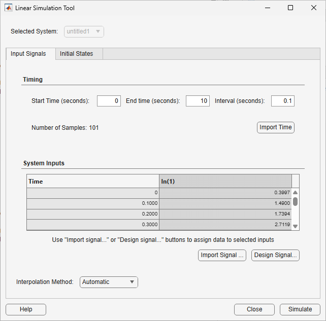
On the Input Signals tab, in the Timing section, specify the time vector for your signal.
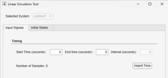
To do so, you can:
Specify the start time, end time, and sampling interval.
Import the time vector from the MATLAB workspace.
To manually specify the time vector, enter the following values in seconds.
Start Time — Simulation start time, specified as a numeric value.
End Time — Simulation end time, specified as a numeric value greater than the sum of the start time and sampling interval.
Interval — Sampling interval, specified as a positive numeric value.
When you modify any of these values, the software automatically adjusts the end time such that it is equal to the start time plus a multiple of the sampling interval.
To import a time vector, click Import Time.
In the Import Time dialog box, the table shows any variables in the MATLAB workspace that are row or column vectors.

In the table, select a vector to import. The vector must be uniformly sampled with a positive sampling interval.
Click Import.
Once you define a time vector, the Number of Samples field shows how many samples it contains. This value must match the length of any input signals that you define.
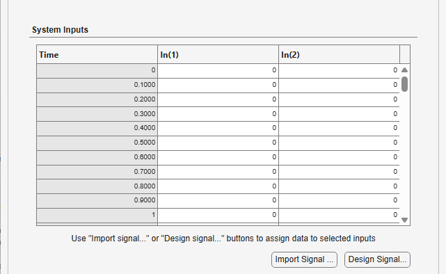
Also, the System Inputs table shows the specified time vector in the first column. The remaining columns correspond to the input signals for your dynamic system model.
To import signal data from a file, first import the data to the MATLAB workspace. For more information on importing data from files, see Supported File Formats for Import and Export.
Specify a time vector. For more information, see Specify Time Vector.
On the Input Signals tab, the System Inputs table shows the specified time vector in the first column. The remaining columns contain the input signals for your dynamic system model.
Click the input column for which you want to import signal data.
Click Import Signal.
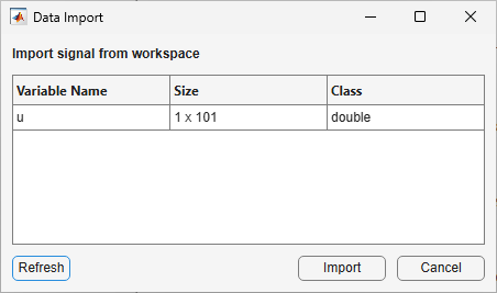
In the Data Import dialog box, the table shows any variables in the MATLAB workspace that are row or column vectors and that have a length equal to the number of samples in your specified time vector.
Select a variable from the table and click Import.
In the System Inputs table, the selected data column updates to show the imported signal values. You can manually edit the values in the System Inputs table.
For multi-input systems, select columns and import signal data for each input channel separately.
To import the same input signal into multiple input channels, you can select multiple signals in the System Inputs table by holding Ctrl while clicking signals. When you do so, the software copies the imported input signal to all selected inputs channels.
You can generate arbitrary input signals in the form of a sine wave, square wave, step function, or white noise.
Specify a time vector. For more information, see Specify Time Vector.
On the Input Signals tab, the System Inputs table shows the specified time vector in the first column. The remaining columns contain the input signals for your dynamic system model. The number of columns equals the number of model inputs.
Click one or more input columns for the channel for which you want to design an input signal. To select multiple signals, hold Ctrl while clicking signals. If you select multiple columns, each signal is set to the same designed signal.
Click Design Signal.
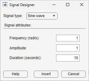
In the Signal Designer dialog box, select the type of signal to create and specify the signal parameters.
To create a sine wave, under Signal type, select
Sine wave and specify these signal parameters:
Frequency — Signal frequency in
rad/TimeUnit, whereTimeUnitis the is the time unit of the specified dynamic system modelAmplitude — Signal amplitude
Duration — Signal duration in the time unit of the specified dynamic system model
To create a square wave, under Signal type, select
Square wave and specify these signal parameters:
Frequency — Signal frequency in
rad/TimeUnit, whereTimeUnitis the is the time unit of the specified dynamic system modelAmplitude — Signal amplitude
Duration — Signal duration in the time unit of the specified dynamic system model
To create a step function, under Signal type, select
Step function wave and specify these signal
parameters:
Starting level — Initial signal value
Step size — Amplitude of the step size
Transition time — Time of the step transition in seconds
Duration — Signal duration in the time unit of the specified dynamic system model
To create a white noise signal, under Signal type, select
White noise and specify these signal parameters:
Mean — Average signal value
Standard deviation — Standard deviation of the signal
Probability density — Select whether to generate Gaussian or uniform white noise.
Duration — Signal duration in the time unit of the specified dynamic system model
For all signals, if you specify a duration that is less than the length of your time vector, the software pads the input signal with zeros.
Click Insert.
In the System Inputs table, the selected data columns update to show the designed signal values. You can manually edit the values in the System Inputs table.
If your system is a state-space model, you can specify initial state values for the simulation.
On the Initial States tab, in the Specify Initial States table, you can manually specify initial values for each state in your system.
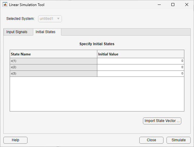
To do so, specify the state value in the Initial Value column.
You can also import initial conditions by clicking Import State Vector.
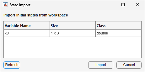
In the State Import dialog box, the table lists any variables in the MATLAB workspace that are vectors with length equal to the number of states in your system.
Select a variable from the table and click Import.