Optimize CSI Feedback Autoencoder Training Using MATLAB Parallel Server and Experiment Manager

Since R2024a

This example shows how to accelerate determining the optimal training hyperparameters of an autoencoder model that simulates channel state information (CSI) compression. To speed up this process, the example uses a MATLAB® Parallel Server™ and the Experiment Manager app.

Using a Cloud Center cluster can significantly reduce the hyperparameter search time for training a neural network. For example, with a 40-worker GPU cluster, this example can achieve a 32x speedup as compared to a single local GPU machine with the same specifications.

For more information about using an autoencoder for CSI compression, see CSI Feedback with Autoencoders.

Generate Training Data

Prepare and preprocess a data set of clustered delay line (CDL) channel estimates to train the autoencoder. For information on how the training data set is generated, refer to the Prepare Data in Bulk section of the CSI Feedback with Autoencoders Example.

You have the choice of downloading a pregenerated training data set or generating the data set by using the helperCSINetCreateDataset function.

downloadDataset = "yes";
if strcmp(downloadDataset,"yes")
    dataFullPath = matlab.internal.examples.downloadSupportFile("comm","CSIDataset.zip");
    unzip(dataFullPath, fullfile(exRoot(),"CSIDataset"));
    movefile(dataFullPath);
else
    helperCSINetCreateDataset(exRoot); %#ok
end

Optimize Hyperparameters with Experiment Manager

The Experiment Manager app allows you to create deep learning experiments to train neural networks under multiple initial conditions and compare the results. In this example, you use Experiment Manager to sweep through a range of training hyperparameter values to determine the optimal training options.

Extract the preconfigured project CSITrainingEM.mlproj.

if ~exist("CSITrainingEM","dir")
  projRoot = helperCSINetExtractProject("CSITrainingEM");
end

Open the .\CSITrainingEM\CSITrainingEM.prj project in Experiment Manager.

The Optimize Hyperparameters experiment uses a Bayesian optimization strategy with the hyperparameter search ranges specified below. Specify CSIAutoEncNN_setup as the experiment setup function to define the training data, the autoencoder architecture, and the training options for the experiment. Specify E2E_NMSE as a post-training custom metric to compute after each training trial, where E2E_NMSE is the normalized mean square error (NMSE) between the autoencoder's inputs and outputs in decibels (dB). The NMSE in dB is a typical metric for measuring the performance of CSI feedback autoencoders. For additional details on this custom metric, see the End-to-End CSI Feedback System section of CSI Feedback with Autoencoders Example.

Run Trials on a Parallel Cluster

The execution mode in Experiment Manager is set to Sequential, which runs one trial at a time. This mode can be time-consuming if the number of trials is large or each trial takes a long time to run. To reduce execution time, set the mode to Simultaneous to run multiple trials in parallel with Parallel Computing Toolbox™.

Although you can create a parallel cluster using the CPU processors on your local desktop, training neural networks on a local pool of CPU workers is often too slow. Instead, use a parallel cluster with access to multiple GPUs.

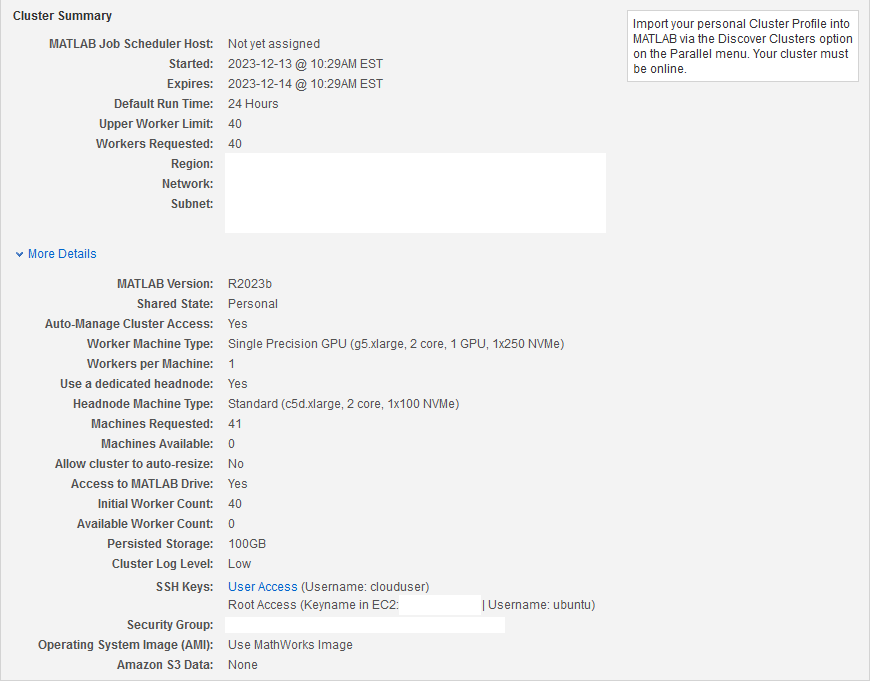
Create Cloud Cluster

Create a cloud cluster using Cloud Center. For topics to help you begin working with Cloud Center, see Getting Started with Cloud Center. To create a cluster, follow the instructions in Create and Discover Clusters.

The cluster has 40 workers, each with access to a GPU.

Access Cloud Center Cluster from MATLAB

Use the Discover Clusters wizard to find and connect to your Cloud Center cluster from MATLAB. To learn more, see Discover Clusters.

If the wizard finds a cloud cluster, it automatically sets it as the default cluster. Alternatively, you can specify the name of your cloud cluster profile as an input to the parcluster (Parallel Computing Toolbox) function. Create a cluster object and start a parallel pool.

c = parcluster;
if ~isempty(gcp("nocreate"))
    delete(gcp("nocreate"));
end
p = parpool(c);

Starting parallel pool (parpool) using the 'Processes' profile ...
14-Mar-2024 16:12:20: Job Queued. Waiting for parallel pool job with ID 3 to start ...
Connected to parallel pool with 6 workers.

Copy Training Data Set to the Cloud

When you use the parallel cluster to run your trials, the workers in the cloud will need access to your training data. Cloud workers have no access to your personal machine. You need to put the training data at a location accessible to the workers.

Define the path to the dataset ZIP file.

datasetZipFile = fullfile(exRoot(),"CSIDataset.zip");

You can copy the data set file to the /shared/tmp area of the parallel cluster.

However, if you want the data to persist on the cluster after you shut it down and restart it, copy the data to /shared/persisted/ instead of /shared/tmp/.

First, define the MATLAB job scheduler host name (available from your cluster details on Cloud Center). You can also get the host name using the Host property of the cluster object.

jobSchedulerHost = c.Host;

Next, download an SSH key identity file to transfer the data. For information on how to download the key, refer to Download SSH Key Identity File.

Then define the path to your SSH key identity file.

SSHKeyPath = "pathToPEMFile";

To copy the data set file to /shared/tmp on the cluster, from a command shell, execute this command:

command = sprintf("scp -i %s %s ubuntu@%s:/shared/tmp/",SSHKeyPath,datasetZipFile,jobSchedulerHost);

Using one worker from the pool, unzip the data set.

parfeval(@()unzip('/shared/tmp/CSIDataset.zip','/shared/tmp/'),1);

Copy Source Code to Cloud

For the experiment to run, your cluster must also have access to the helper files of this example.

Attach your files to the parallel pool by using the addAttachedFiles (Parallel Computing Toolbox) function.

filesToCopy = {'helperCSINetAddResidualLayers.m', ...           
  'helperCSINetChannelEstimate.m', ...
  'helperCSINetDecode.m', ...                          
  'helperCSINetEncode.m', ...                          
  'helperCSINetDLNetwork.m',...                      
  'helperCSINetPostprocessChannelEstimate.m', ...     
  'helperCSINetPreprocessChannelEstimate.m', ...       
  'helperCSINetSplitEncoderDecoder.m', ...   
  'helperCSINetGetDatastore.m', ...
  'helperNMSE.m'};

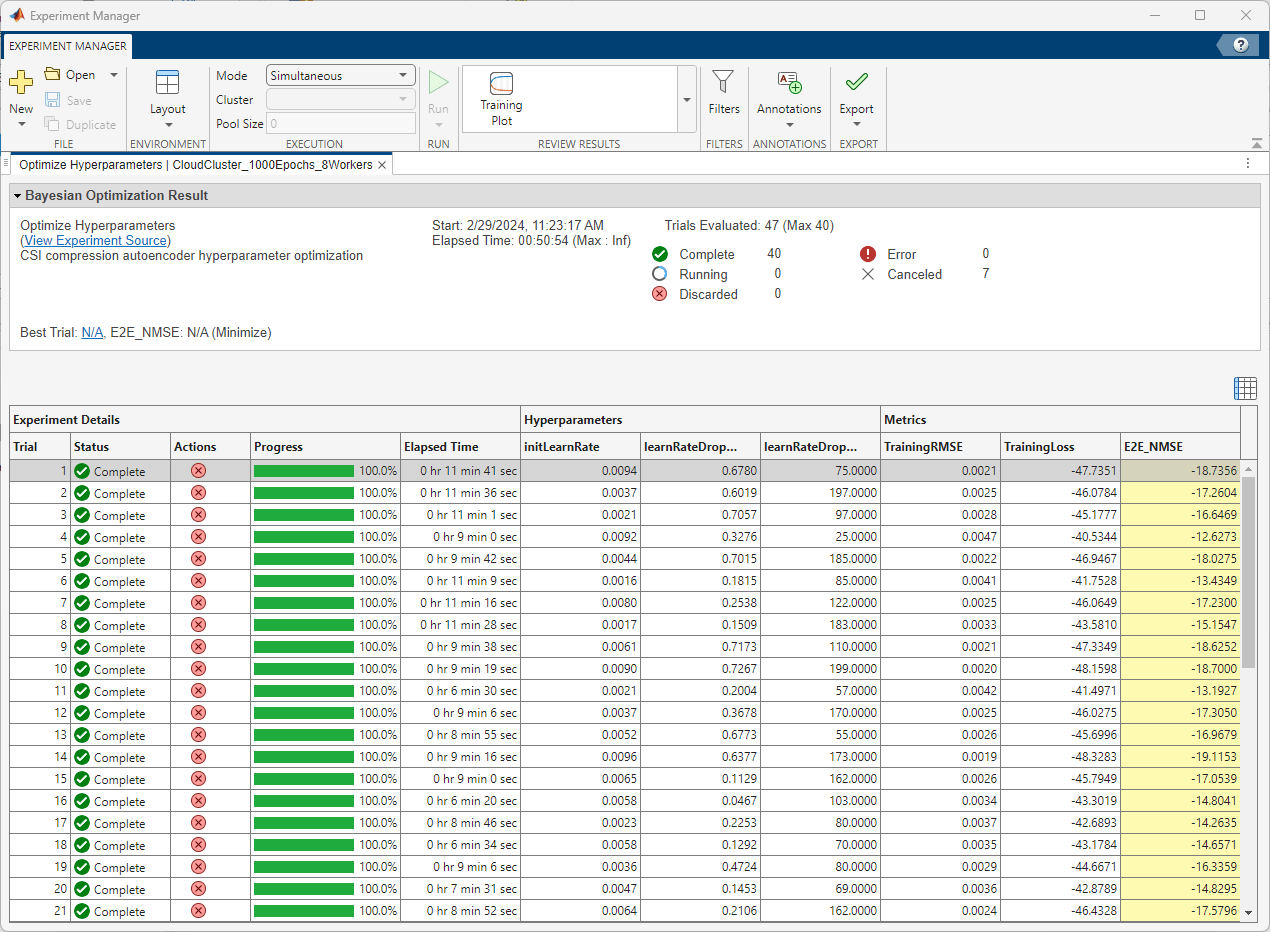
addAttachedFiles(p,filesToCopy);

Run Experiment on Cloud

After running the experiment on the cloud cluster, Experiment Manager shows you the run time of the whole experiment as well as the run time of each trial in the results table. The table also highlights the set of hyperparameters resulting in the minimum validation RMSE and the corresponding E2E_NMSE value. Using the cloud cluster in this example, each trial runs on a worker with a single GPU.

Results

The following results are based on running the same experiment in three different scenarios:

• Using a parallel cluster with one worker.

• Using a parallel cluster with 8 workers.

• Using a parallel cluster with 40 workers.

For these scenarios, each worker is a g5.xlarge, 2 core, 1 GPU, 1x250 NVMe machine. Each worker has an NVIDIA® A10G Tensor Core GPU with 24 GB GPU memory.

The one-worker cluster serves as the baseline which represents running the experiment trials sequentially on a single machine.

All experiments use the Bayesian optimization strategy, with a maximum number of trials equal to 40.

Training for 1000 Epochs

Running the experiment while training the network for 1000 epochs in each trial shows these results:

Number of Workers	Experiment Execution Time (hh:mm:ss)	Speedup Factor
1	06:00:40	Baseline
8	00:50:47	7.10
40	00:12:28	28.93

Running the 40 trials sequentially on one GPU machine takes 6 hours to complete. Using multi-machine GPU clusters reduces the linear run time substantially.

Although the speedups are significant, they are lower than the theoretical highest achievable speedup. For example, with a 40-worker cluster, the speedup is 28.93x, which is lower than the 40x theoretical upper bound (1x speedup for each worker). You do not achieve the upper bound because of the overhead introduced by the cluster, where a single host machine processes the responses from all individual workers.

Training For 3000 Epochs

To reduce the effect of the cluster overhead, execute the experiment again with each trial running for 3000 epochs instead of 1000 epochs.

Number of workers	Experiment Execution Time (hh:mm:ss)	Speedup Factor
1	18:20:00	Baseline
8	2:22:21	7.72
40	00:34:20	32.03

Executing trials sequentially on a single machine now takes over 18 hours. This corresponds to a single trial run time of about 27.5 minutes.

The experiment execution time is 34 minutes on a 40-worker cluster. Since the experiment has 40 trials, all the trials run simultaneously, and the experiment run time approaches the run time of a single trial (plus overhead). The speedup factor of 32.03 is now closer to the theoretical speedup factor of 40.

Conclusion

By leveraging a 40-worker parallel cluster to run the experiment, you approach the theoretical speedup factor of 40 compared to a baseline where you run trials in sequential mode with a single GPU machine of comparable strength.

Local Functions

The exRoot function returns the root directory of this example in rootDir.

function rootDir = exRoot()
rootDir = fileparts(which("helperCSINetDLNetwork"));
end