Offline Training and Testing of PyTorch Model for CSI Feedback Compression
This example shows how to perform offline training and testing of a PyTorch® autoencoder based neural network for channel state information (CSI) feedback compression.
In this example, you:
Train an autoencoder-based neural network.
Test the trained neural network.
Compare the performance metrics of the complex input lightweight neural network (CLNet) PyTorch model across multiple compression factors.
Introduction
In 5G networks, efficient handling of CSI is crucial for optimizing downlink data transmission. Traditional methods rely on feedback mechanisms where the user equipment (UE) processes the channel estimate to reduce the CSI feedback data sent to the access node (gNB). However, an innovative approach involves using an autoencoder-based neural networks to compress and decompress the CSI feedback more effectively.
In this example, you define, train, test, and compare the performance of the following autoencoder model:
Complex input lightweight neural network (CLNet): CLNet is a lightweight neural network designed for massive multiple-input multiple-output (MIMO) CSI feedback, which utilizes complex-valued inputs and attention mechanisms to improve accuracy while reducing computational overhead [1].
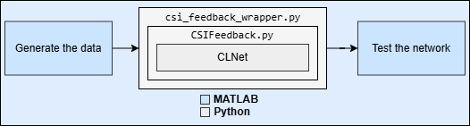
This is example is the step three in a series of examples that takes you through a CSI feedback compression workflow. You can run each step independently or work through the steps in order. This example follows the Preprocess Data for AI-Based CSI Feedback Compression example that shows how to preprocess the channel estimates.
Load the preprocessed channel estimates data. If you have run the previous step, then the example uses the data that you prepared in the previous step. Otherwise, the example prepares the data as shown in the Preprocess Data for AI-Based CSI Feedback Compression example.
if ~exist("inputData","var") || ~exist("systemParams","var") || ~exist("dataOptions","var") || ~exist("channel","var") || ~exist("carrier","var") numSamples =1500; [inputData,systemParams,dataOptions,channel,carrier] = prepareData(numSamples); end
Starting channel realization generation
6 worker(s) running
00:00:10 - 100% Completed
Starting CSI data preprocessing
6 worker(s) running
00:00:01 - 100% Completed
Channel configuration is as follows.
channel
channel =
  nrCDLChannel with properties:

                 DelayProfile: 'CDL-C'
                 AngleScaling: false
                  DelaySpread: 3.0000e-07
             CarrierFrequency: 4.0000e+09
          MaximumDopplerShift: 5
          UTDirectionOfTravel: [2×1 double]
                   SampleRate: 15360000
         TransmitAntennaArray: [1×1 struct]
     TransmitArrayOrientation: [3×1 double]
          ReceiveAntennaArray: [1×1 struct]
      ReceiveArrayOrientation: [3×1 double]
           NormalizePathGains: true
                SampleDensity: 64
                  InitialTime: 0
                 RandomStream: 'Global stream'
      NormalizeChannelOutputs: true
             ChannelFiltering: false
               NumTimeSamples: 15360
               OutputDataType: 'single'
    TransmitAndReceiveSwapped: false
                       UseGPU: 'off'
        ChannelResponseOutput: 'ofdm-response'
Carrier configuration is as follows.
carrier
carrier =
  nrCarrierConfig with properties:

                NCellID: 1
      SubcarrierSpacing: 15
           CyclicPrefix: 'normal'
              NSizeGrid: 52
             NStartGrid: 0
                  NSlot: 0
                 NFrame: 0
    IntraCellGuardBands: [0×2 double]

   Read-only properties:
         SymbolsPerSlot: 14
       SlotsPerSubframe: 1
          SlotsPerFrame: 10
The inputData variable contains samples of -by- -by- 2 arrays.
[maxDelay,nTx,Niq,Nsamples] = size(inputData)
maxDelay =
28
nTx =
8
Niq =
2
Nsamples =
1500
Set Up Python Environment
Set up the Python® environment as described in Call Python from MATLAB for Wireless before running the example. Specify the full path of the Python executable to use below. The helperSetupPyenv function sets the Python Environment in MATLAB® based on the selected options and checks that the libraries listed in the requirements_csi_feedback.txt file are installed.
If you use Windows®, provide the path to the pythonw.exe file.
if ispc exePath = ".venv\Scripts\pythonw.exe"; else exePath = "../python/python/bin/python3"; end exeMode ="OutOfProcess"; currentPenv = helperSetupPyenv(exePath,exeMode,"requirements_csi_feedback.txt");
Setting up Python environment
Parsing requirements_csi_feedback.txt
Checking required package 'numpy'
Checking required package 'torch'
Required Python libraries are installed.
Split Data Set into Training, Validation, and Testing Data
Split the prepared data into training, validation and testing datasets. In this example, you use the helperCSISplitData function to split the prepared data in to a ratio of 10:3:2, where 10,3 and 2 correspond to training, validation, and testing splits.
splitRatio =[10,3,2]; % Split ratio for training, validation and testing [HTrain, HValid, HTest] = helperCSISplitData(inputData,splitRatio);
Normalize Data Set
Normalize the data set to achieve zero mean and a target standard deviation of 0.0212, restricting most values to the range of [-0.5, 0.5].
[HTrain, HValid, HTest, norm] = helperCSINormalizeData(HTrain, HValid, HTest);
Define Neural Network
Next, define the CSI feedback autoencoder.
Specify the autoencoder-based neural network.
autoencoderNetwork = "CLNet";Select a compression factor. Increasing the compression factor decreases the accuracy of the decompressed output because the network retains less information.
compressionFactor =  4;
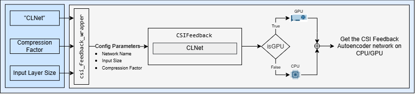
4;Call the method in the Python wrapper file csi_feedback_wrapper.py to initialize and return the network using the specified parameters. It acts as an interface between MATLAB and Python.
inputLayerSize = size(HTrain);  % Input layer size is calculated from the prepared data
pyCSINN = py.csi_feedback_wrapper.construct_model(autoencoderNetwork, inputLayerSize, compressionFactor);
Train Neural Network
Set the training parameters to optimize the network performance. Set the maxEpochs to 1000 and numSamples to 150000 here to ensure complete training of the network.
initialLearningRate  = 0.0001; % Enter initial learning rate for training
maxEpochs            = 2;      % Number of epochs for training
miniBatchSize        = 1000;   % Mini-batch size for training
Use train method in Python wrapper file to set up the trainer with the training parameters in Python and train the PyTorch model.
results = py.csi_feedback_wrapper.train(...
pyCSINN, ...
HTrain, HValid, HTest, ...
initialLearningRate, ...
maxEpochs, ...
miniBatchSize);
Epoch: 1
I 11:57:49] => Train  Loss: 3.080e-02


=! Best Validation rho: 4.718e-01 (Corresponding nmse=1.916e+01; epoch=1)
   Best Validation NMSE: 1.916e+01 (Corresponding rho=4.718e-01;  epoch=1)

Epoch: 2
I 11:57:49] => Train  Loss: 2.952e-02


=! Best Validation rho: 4.737e-01 (Corresponding nmse=1.894e+01; epoch=2)
   Best Validation NMSE: 1.894e+01 (Corresponding rho=4.737e-01;  epoch=2)
trainedNet = results{1};
training_loss = results{2};
validation_loss = results{3};
Test Neural Network
Use the predict method to process the test data.
tic;
HPredReal = single(py.csi_feedback_wrapper.predict(trainedNet,HTest));
elapsedTime = toc;
Calculate the correlation and normalized mean squared error (NMSE) between the input and output of the autoencoder network.
The correlation is defined as
where, is the channel estimate at the input of the autoencoder and is the channel estimate at the output of the autoencoder.
NMSE is defined as
where, is the channel estimate at the input of the autoencoder and is the channel estimate at the output of the autoencoder.
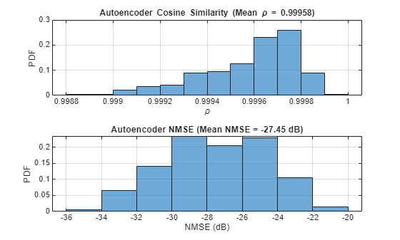
HTestComplex = squeeze(complex(HTest(:,:,1,:), HTest(:,:,2,:)));
HPredComplex = squeeze(complex(HPredReal(:,:,1,:), HPredReal(:,:,2,:)));
rho = abs(helperComplexCosineSimilarity(HTestComplex, HPredComplex)); % Compute complex cosine similarity
meanRho = mean(rho);
[nmse,meanNmse] = helperCSINMSELossdB(HTestComplex, HPredComplex);    % Compute NMSE
helperPlotMetrics(rho, meanRho, nmse, meanNmse);
metricsTable = table(autoencoderNetwork, compressionFactor, meanNmse, meanRho, ...
  elapsedTime, single(py.csi_feedback_wrapper.info(pyCSINN)), ...
    'VariableNames', {'Model', 'Compression Factor', 'NMSE(dB)', ...
    'Rho', 'InferenceTime', 'NumberOfLearnables'});
disp(metricsTable)
     Model     Compression Factor    NMSE(dB)      Rho      InferenceTime    NumberOfLearnables
    _______    __________________    ________    _______    _____________    __________________

    "CLNet"            4             -27.691     0.99958      0.035358           1.0289e+05
Save Trained Network
Enable saveNetwork to save the trained model in a PT file with the filename as checkPointName.
saveNetwork =true; if saveNetwork % Save the trained network checkPointName = autoencoderNetwork+string(compressionFactor); py.csi_feedback_wrapper.save(trainedNet,checkPointName,autoencoderNetwork, inputLayerSize, compressionFactor); end
Compare Networks
The following table compares the performance metrics, inference time, and learnable parameters of CLNet across compression factors 4, 16, and 64.
Model | Compression Factor | NMSE(dB) | Rho | Inference Time | Number of Learnables |
|---|---|---|---|---|---|
CLNet | 4 | -46.639 | 0.99999 | 0.14911 | 1.0289e05 |
CLNet | 16 | -44.06 | 0.99998 | 0.18851 | 27538 |
CLNet | 64 | -35.524 | 0.99983 | 0.15048 | 8701 |
Further Exploration
In this example, you train and test the PyTorch network, CLNet using offline training. The CSI feedback autoencoder architecture achieves comparable NMSE and cosine similarity performance across different compression ratios. Adjust the data generation parameters and optimize hyperparameters for your specific use case.
For more information about online training and throughput analysis, see these examples:
References
[1] Ji, S., & Li, M. (2021). CLNet: Complex Input Lightweight Neural Network Designed for Massive MIMO CSI Feedback. IEEE Wireless Communications Letters, 10(10), 2318–2322. doi:10.1109/lwc.2021.3100493.
Helper Functions
helperSetupPyenv.mhelperinstalledlibs.pyhelperLibraryChecker.mhelperCSIDownloadFiles.mhelperCSIGenerateData.mhelperCSIChannelEstimate.mhelperCSIPreprocessChannelEstimate.mhelperCSISplitData.mCSIFeedback.pyclnet.pycsi_feedback_wrapper.pyhelperCSINMSELossdB.mhelperNMSE.mhelperComplexCosineSimilarity.m
PyTorch Wrapper Template
You can use your own PyTorch models in MATLAB using the Python interface. The py_wrapper_template.py file provides a simple interface with the following predefined API:
model_under_test: returns the PyTorch neural network modeltrain: trains the PyTorch modelsetup_trainer: sets up a trainer object for with online trainingtrain_one_iteration: trains the PyTorch model for one iteration for online trainingvalidate: validates the PyTorch model for online trainingpredict: runs the PyTorch model with the provided input(s)save: saves the PyTorch model and metadataload: loads the PyTorch modelinfo: prints or returns information on the PyTorch model
You can modify the py_wrapper_template.py file. Follow the instruction in the template file to implement the recommended entry points. Use the entry point functions as shown in this example to use your own PyTorch models in MATLAB.
Local Functions
function [inputData,systemParams,dataOptions,channel,carrier] = prepareData(numSamples) carrier = nrCarrierConfig; nSizeGrid = 52; % Number resource blocks (RB) systemParams.SubcarrierSpacing =15; % 15, 30, 60, 120 kHz carrier.NSizeGrid = nSizeGrid; carrier.SubcarrierSpacing = systemParams.SubcarrierSpacing; waveInfo = nrOFDMInfo(carrier); systemParams.TxAntennaSize = [2 2 2 1 1]; % rows, columns, polarization, panels systemParams.RxAntennaSize = [2 1 1 1 1]; % rows, columns, polarization, panels systemParams.MaxDoppler = 5; % Hz systemParams.RMSDelaySpread = 300e-9; % s systemParams.DelayProfile =
"CDL-C"; % CDL-A, CDL-B, CDL-C, CDL-D, CDL-D, CDL-E systemParams.NumSubcarriers = carrier.NSizeGrid*12; channel = nrCDLChannel; channel.DelayProfile = systemParams.DelayProfile; channel.DelaySpread = systemParams.RMSDelaySpread; % s channel.MaximumDopplerShift = systemParams.MaxDoppler; % Hz channel.RandomStream = "Global stream"; channel.TransmitAntennaArray.Size = systemParams.TxAntennaSize; channel.ReceiveAntennaArray.Size = systemParams.RxAntennaSize; channel.ChannelFiltering = false; channel.SampleRate = waveInfo.SampleRate; samplesPerSlot = ... sum(waveInfo.SymbolLengths(1:waveInfo.SymbolsPerSlot)); channel.NumTimeSamples = samplesPerSlot; % 1 slot worth of samples systemParams.NumSymbols = 14; useParallel =
true; saveData =
true; dataDir = fullfile(pwd,"Data"); dataFilePrefix = "CH_est"; numSlotsPerFrame = 1; resetChannel = true; numFrames = numSamples / prod(systemParams.RxAntennaSize); sdsChan = helper3GPPChannelRealizations(... numFrames, ... channel, ... carrier, ... UseParallel=useParallel, ... SaveData=saveData, ... DataDir=dataDir, ... dataFilePrefix=dataFilePrefix, ... NumSlotsPerFrame=numSlotsPerFrame, ... ResetChannelPerFrame=resetChannel); dataOptions.DataDomain =
"Frequency-Spatial (FS)"; dataOptions.TruncationFactor =
10; Tdelay = 1/(systemParams.NumSubcarriers*carrier.SubcarrierSpacing*1e3); rmsDelaySpreadSamples = channel.DelaySpread/Tdelay; [data,dataOptions] = helperPreprocess3GPPChannelData( ... sdsChan, ... TrainingObjective = "autoencoding", ... AverageOverSlots = true, ... TruncateChannel = true, ... ExpectedDelaySpreadSamples = rmsDelaySpreadSamples, ... TruncationFactor = dataOptions.TruncationFactor, ... DataComplexity = "real (2D)", ... IQDimension = 3, ... DataDomain = dataOptions.DataDomain, ... UseParallel = useParallel, ... SaveData = false); meanVal = mean(data{1},'all'); stdVal = std(data{1},[],'all'); inputData = (data{1}-meanVal) / stdVal; targetStd = 0.0212; inputData = inputData*targetStd+0.5; systemParams.Normalization = "mean-variance"; systemParams.MeanValue = meanVal; systemParams.StandardDeviationValue = stdVal; systemParams.TargetStandardDeviation = targetStd; systemParams.ExpectedDelaySpreadSamples = dataOptions.ExpectedDelaySpreadSamples; end function varargout = helperCSINormalizeData(varargin) %helperCSINormalizeData Normalize the given inputs and return the %normalization parameters H = cat(4,varargin{:}); meanValue = mean(H,'all'); stdValue = std(H,[],'all'); targetStd = 0.0212; for i=1:numel(varargin) varargout{i} = (varargin{i}-meanValue)/stdValue*targetStd+0.5; end norm.MeanVal = meanValue; norm.StdValue = stdValue; norm.TargetSTDValue = targetStd; varargout{i+1} = norm; end function helperPlotMetrics(rho,meanRho,nmse,meanNmse) %helperPlotMetrics Plot the histograms for RHO and NMSE values figure tiledlayout(2,1) nexttile histogram(rho,"Normalization","probability") grid on title(sprintf("Autoencoder Cosine Similarity (Mean \\rho = %1.5f)", ... meanRho)) xlabel("\rho"); ylabel("PDF") nexttile histogram(nmse,"Normalization","probability") grid on title(sprintf("Autoencoder NMSE (Mean NMSE = %1.2f dB)",meanNmse)) xlabel("NMSE (dB)"); ylabel("PDF") end