Read, Analyze, and Process SOFA Files
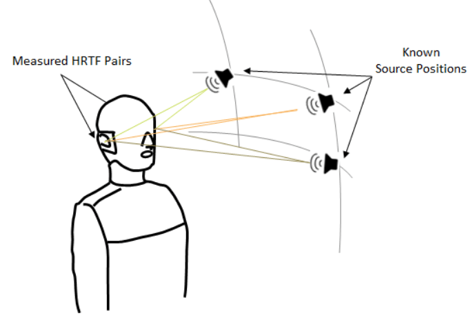
SOFA (Spatially Oriented Format for Acoustics) [1] is a file format for storing spatially oriented acoustic data like head-related transfer functions (HRTF) and binaural or spatial room impulse responses. SOFA has been standardized by the Audio Engineering Society (AES) as AES69-2015.
In this example, you load a SOFA file containing HRTF measurements for a single subject in MATLAB®. You then analyze the HRTF measurements in the time domain and the frequency domain. Finally, you use the HRTF impulse responses to spatialize an audio signal in real time by modeling a moving source based on desired azimuth and elevation values.
Explore a SOFA File in MATLAB
You use a SOFA file from the SADIE II database [2]. The file corresponds to spatially discrete free-field in-the-ear HRTF measurements for a single subject. The measurements characterize how each ear receives a sound from a point in space.
Download the SOFA file.
downloadFolder = matlab.internal.examples.downloadSupportFile("audio","SOFA/SOFA.zip");
dataFolder = tempdir;
unzip(downloadFolder,dataFolder)
netFolder = fullfile(dataFolder,"SOFA");
addpath(netFolder)
filename = "H10_48K_24bit_256tap_FIR_SOFA.sofa";
Display SOFA File Contents
SOFA files consist of binary data stored in the netCDF-4 format. You can use MATLAB to read and write netCDF files.
Display the contents of the SOFA file using ncdisp (execute ncdisp(filename)).
The file contents consist of multiple fields corresponding to different aspects of the measurements, such as the (fixed) listener position, the varying source position, the coordinate system used to capture the data, general metadata related to the measurement, as well as the measured impulse responses.
NetCDF is a "self-describing" file format, where data is stored along with attributes that can be used to assist in its interpretation. Consider the display snippet corresponding to the source position for example:
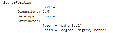
SourcePosition contains the coordinates for the varying source position used in the measurements (here, there are 2114 separate positions). The file also contains attributes (Type, Units) describing the coordinate system used to store the positions (here, spherical), as well as information about the dimensions of the data (C,M). The dimensions are defined in the AES69 standard [3]:
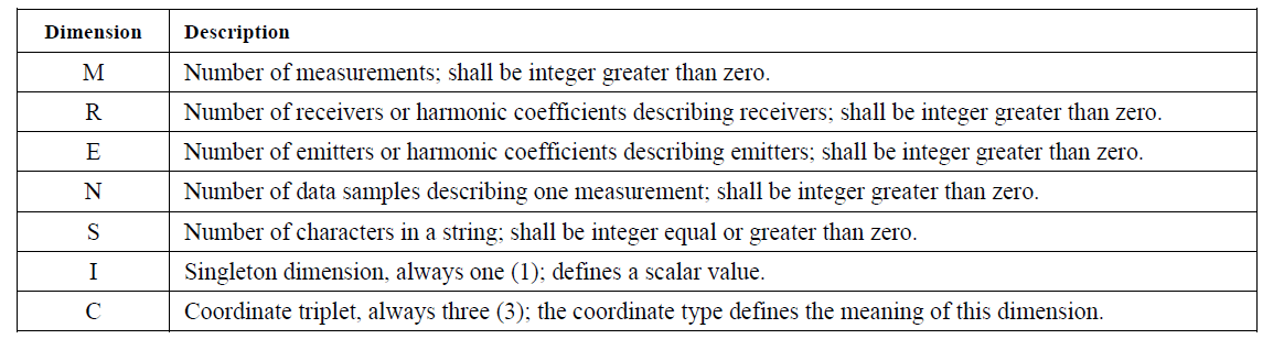
For the file in this example:
M = 2114 (the total number of measurements, each corresponding to a unique source position).
R = 2 (corresponding to the two ears).
E = 1 (one emitter or sound source per measurement).
N = 256 (the length of each recorded impulse response).
Read SOFA File Information
Use ncinfo to get information about the SOFA file.
SOFAInfo = ncinfo(filename);
The fields of the structure SOFAInfo hold information related to the file's dimensions, variables and attributes.
Read a Variable from the SOFA File
Use ncread to read the value of a variable in the SOFA file.
Read the variable corresponding to the measured impulse responses.
ir = ncread(filename,"Data.IR");
size(ir)
ans = 1×3
256 2 2114
This variable holds impulse responses for the left and right ear for 2114 independent measurements. Each impulse response is of length 256.
Read the sampling rate of the measurements.
fs = ncread(filename,"Data.SamplingRate")fs = 48000
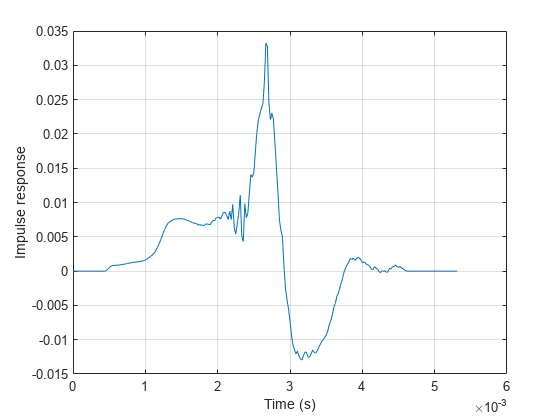
Plot the first measured impulse response.
figure;
t = (0:size(ir,1)-1)/fs;
plot(t,ir(:,1,1))
grid on
xlabel("Time (s)")
ylabel("Impulse response")
Read SOFA Files with sofaread
It is possible to read and analyze the contents of the SOFA file using a combination of ncinfo and ncread. However, the process can be cumbersome and time consuming.
The function sofaread allows you to read the entire contents of a SOFA file in one line of code.
Use sofaread to get the contents of the SOFA file.
s = sofaread(filename)
s =
  audio.sofa.SimpleFreeFieldHRIR handle with properties:

            Numerator: [2114×2×256 double]
                Delay: [0 0]
         SamplingRate: 48000
    SamplingRateUnits: "hertz"

  Show all properties
Click "Show all properties" in the display above to see the rest of the properties from the SOFA file.
You can easily access the measured impulses responses.
ir = s.Numerator;
size(ir)
ans = 1×3

    2114    2    256
You access other variables in a similar fashion. For example, read the source positions along with the coordinate system used to express them:
srcPositions = s.SourcePosition;
size(srcPositions)
ans = 1×2

    2114    3
srcPositions(1,:)
ans = 1×3

    0    -90.0000    1.2000
s.SourcePositionType
ans =
'spherical'
s.SourcePositionUnits
ans =
"degree, degree, meter"
View the Measurement Geometry
Call plotGeometry to view the general geometric setup of the measurements.
figure;
plotGeometry(s)

Alternatively, specify input indices to restrict the plot to desired source locations. For example, plot the source positions located in the median plane.
figure;
idx = findMeasurements(s,Plane="median");
plotGeometry(s,MeasurementIndex=idx)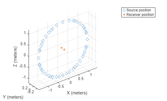
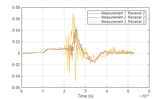
Plot Measurement Impulse Responses
The file in this example uses the SimpleFreeFieldHRIR convention, which stores impulse response measurements in the time domain as FIR filters.
s.SOFAConventions
ans =
"SimpleFreeFieldHRIR"
s.DataType
ans =
"FIR"
Plot the impulse response of the first 3 measurements corresponding to the second receiver using impz.
figure;
impz(s, MeasurementIndex=1:3,Receiver=2)
Compute HRTF Frequency Responses
It is straightforward to compute and plot the frequency response of the impulse responses using freqz.
Compute the frequency response of the first measurement for both ears. Use a frequency response length of 512.
[H,F] = freqz(s, Receiver=1:2, NPoints=512);
H is the complex frequency response array. F is the vector of corresponding frequencies (in Hertz).
size(H)
ans = 1×3

    512    1    2
size(F)
ans = 1×2

    512    1
You can also use freqz to plot the frequency response by calling the function with no output arguments.
Plot the frequency response of the first 3 measurements in the horizontal plane at zero elevation for the first receiver.
figure;
idx = findMeasurements(s, Plane="horizontal");
freqz(s, MeasurementIndex=idx(1:3), Receiver=1)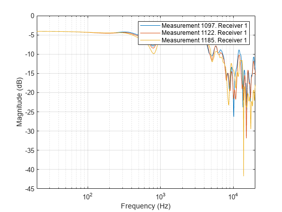
Compute HRTF Spectra
It is often useful to compute and visualize the magnitude spectra of HRTF data in a specific plane in space.
For example, compute the spectrum in the horizontal plane (corresponding to an elevation angle equal to zero) for the first receiver. Use a frequency response length of 2048.
[S,F,azi] = spectrum(s, Plane="horizontal",Receiver=1, NPoints=2048); %#ok
Sis the horizontal plane spectrum of size 2048-by-L, where L is the number of measurements in the specified plane.F is the frequency vector of length 2048.
aziis a vector of length L containing the azimuth angles (in degrees) corresponding to the horizontal plane measurements.
You can plot the spectrum instead of returning it.
figure
spectrum(s, Plane="horizontal",Receiver=1, NPoints=2048);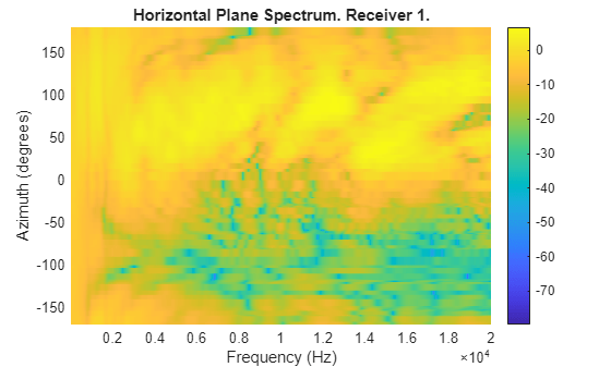
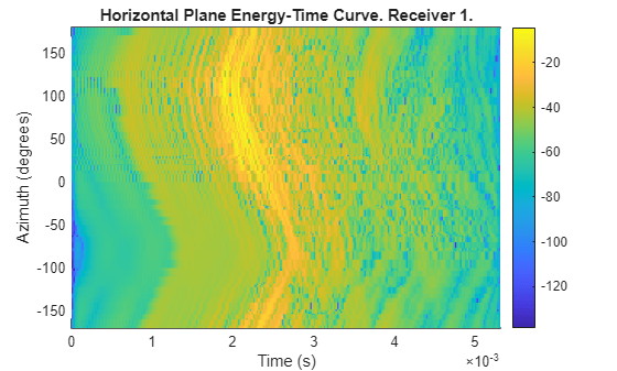
Compute Energy-Time Curve
It is often useful to visualize the decay of the HRTF responses over time using an energy-time curve (ETC).
Measure the ETC in the horizontal plane.
ETC = energyTimeCurve(s);
size(ETC)
ans = 1×2

    256    96
The first dimension of ETC is equal to the length of the impulse response. The second dimension of ETC is equal to the number of points in the specified plane.
Plot the ETC.
figure;
energyTimeCurve(s)
Compute Interaural Time Difference
Interaural time difference (ITD) is the difference in arrival time of a sound between two ears. It is an important binaural cue for sound source localization.
Compute the ITD for all measurements.
ITD = interauralTimeDifference(s, Specification="measurements");Plot the ITD for all measurements.
figure;
interauralTimeDifference(s, Specification="measurements");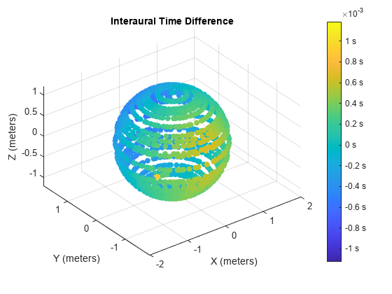
You can also compute and plot the ITD in a specified plane. For example, plot the ITD in the horizontal plane at an elevation of 35 degrees.
figure
interauralTimeDifference(s, Plane="horizontal",PlaneOffsetAngle=35)
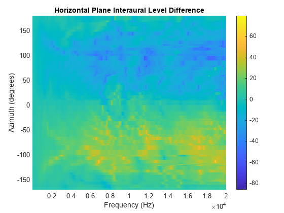
Compute Interaural Level Difference
Interaural level difference (ILD) measures the difference, in decibels, of the received signals at the two ears in the desired plane.
Compute the ILD in the horizontal plane.
[ILD,F] = interauralLevelDifference(s,NPoints=1024);
size(ILD)
ans = 1×2

    1024    96
ILD is 1024-by-L, where L is the number of points in the desired plane.
Plot the ILD in the horizontal plane.
figure
interauralLevelDifference(s)
Compute Frequency Directivity
HRTF measurements are highly frequency selective. It is often useful to compare the received power level of different frequencies in space.
Call directivity to plot the received level at 200 Hz for all measurements.
figure;
directivity(s, 200, Specification="measurements")
Generate a similar plot at 4000 Hz.
figure;
directivity(s, 4000, Specification="measurements")
You can also compute and plot the directivity for selected planes. For example, plot the directivity at 700 Hz and 1200 Hz for the horizontal plane at an elevation of 35 degrees.
figure;
directivity(s, [700 1200], PlaneOffsetAngle=35, Receiver=1)

Interpolate HRTF Measurements
The HRTF measurements in the SOFA file correspond to a finite number of azimuth/elevation angle combinations. It is possible to interpolate the data to any desired spatial location using 3-D HRTF interpolation with interpolateHRTF.
Specify the desired source position (in degrees).
desiredAz = [-120;-60;0;60;120;0;-120;120];
desiredEl = [-90;90;45;0;-45;0;45;45];
desiredPosition = [desiredAz, desiredEl];
Calculate the head-related impulse response (HRIR) using the vector base amplitude panning interpolation (VBAP) algorithm at a desired source position.
interpolatedIR = interpolateHRTF(s, desiredPosition);
You can also visualize the interpolated frequency responses.
figure;
interpolateHRTF(s, desiredPosition);

Model Moving Source Using HRIR Filtering
Filter a mono input through the interpolated impulse responses to model a moving source.
Create an audio file sampled at 48 kHz for compatibility with the HRTF dataset.
desiredFs = s.SamplingRate;
[x,fs] = audioread("Counting-16-44p1-mono-15secs.wav");
y = audioresample(x,InputRate=fs,OutputRate=desiredFs);
y = y./max(abs(y));
audiowrite("Counting-16-48-mono-15secs.wav",y,desiredFs);
Create a dsp.AudioFileReader object to read in a file frame by frame. Create an audioDeviceWriter object to play audio to your sound card frame by frame. Create a dsp.MIMOFIRFilter object. Set the Numerator property to the combined left-ear and right-ear filter pair. Since you want to keep the received signals at each ear separate, set SumFilteredOutputs to false.
fileReader = dsp.AudioFileReader("Counting-16-48-mono-15secs.wav");
deviceWriter = audioDeviceWriter(SampleRate=fileReader.SampleRate);

spatialFilter = dsp.MIMOFIRFilter(squeeze(interpolatedIR(1,:,:)),SumFilteredOutputs=false);
In an audio stream loop:
Read in a frame of audio data.
Feed the audio data through the filter.
Write the audio to your output device. If you have a stereo output hardware, such as headphones, you can hear the source shifting position over time.
Modify the desired source position in 2-second intervals by updating the filter coefficients.
durationPerPosition = 2;
samplesPerPosition = durationPerPosition*fileReader.SampleRate;
samplesPerPosition = samplesPerPosition - rem(samplesPerPosition,fileReader.SamplesPerFrame);

sourcePositionIndex = 1;
samplesRead = 0;
while ~isDone(fileReader)
    audioIn = fileReader();
    samplesRead = samplesRead + fileReader.SamplesPerFrame;

    audioOut = spatialFilter(audioIn);
    deviceWriter(audioOut);

    if mod(samplesRead,samplesPerPosition) == 0
        sourcePositionIndex = sourcePositionIndex + 1;
        spatialFilter.Numerator = squeeze(interpolatedIR(sourcePositionIndex,:,:));
    end
end
As a best practice, release your System objects when complete.
release(deviceWriter)
release(fileReader)
release(spatialFilter);
Spatialize Audio in Real Time
Simulate a sound source moving in the horizontal plane, with an initial azimuth of –90 degrees. Gradually increase the azimuth as the simulation is running.
Compute the starting impulse responses based on the initial source position.
index = 1;
loc = [-90 0];

interpolatedIR = interpolateHRTF(s, ...
    loc);
spatialFilter.Numerator = squeeze(interpolatedIR);
Execute the simulation loop. Shift the source elevation by 30 degrees every 100 loop iterations. Use interpolateHRTF to estimate the new desired impulse responses.
while ~isDone(fileReader)
    index=index+1;
    frame = fileReader();
    frame = frame(:,1);

    audioOut = spatialFilter(frame);

    deviceWriter(audioOut);

    if mod(index,100)==0
        loc(1)=loc(1)+30;
        interpolatedIR = interpolateHRTF(s, ...
            loc);
        spatialFilter.Numerator = squeeze(interpolatedIR);
    end
end
release(deviceWriter)
release(fileReader)
release(spatialFilter);
References
[1] Majdak, P., Zotter, F., Brinkmann, F., De Muynke, J., Mihocic, M., and Noisternig, M. (2022). “Spatially Oriented Format for Acoustics 21: Introduction and Recent Advances,” J Audio Eng Soc 70, 565–584. DOI: 10.17743/jaes.2022.0026.
[2] https://www.york.ac.uk/sadie-project/database.html
[3] Majdak, P., De Muynke, J., Zotter, F., Brinkmann, F., Mihocic, M., and Ackermann, D. (2022). AES standard for file exchange - Spatial acoustic data file format (AES69-2022), Standard of the Audio Engineering Society.
[4] Andreopoulou A, Katz BFG. Identification of perceptually relevant methods of inter-aural time difference estimation. J Acoust Soc Am. 2017 Aug;142(2):588. DOI: 10.1121/1.4996457. PMID: 28863557.
See Also
sofaread | sofawrite | interpolateHRTF