Understanding the Radar Equation | Understanding Radar Principles - MATLAB & Simulink
Video Player is loading.
Current Time 0:00
Duration 18:07
Loaded: 0%
Stream Type LIVE
Remaining Time 18:07
 
1x
  • Chapters
  • descriptions off, selected
  • en (Main), selected
    Video length is 18:07

    Understanding the Radar Equation | Understanding Radar Principles

    From the series: Understanding Radar Principles

    Learn how the radar equation combines several of the main parameters of a radar system in a way that gives you a general understanding of how the system will perform.

    The radar equation is a function of transmit power, antenna gain, transmit frequency, radar cross-section of the object, and the propagation through the environment and radar components. Walk through each of these steps and watch a demonstration of how they contribute to the total received power of the reflected signal back at the radar.

    Published: 13 Jun 2022

    Welcome back to our discussion on the basics of radar. In this video, we're going to focus on radar power and noise. And to do that, I want to introduce the radar equation. The radar equation is a good tool in the early stages of radar design because it combines several of the main parameters of a radar system in a way that gives you a general understanding of how the system will perform.

    I think this is going to be a nice visual introduction to the equation, so I hope you stick around for it. I'm Brian. And welcome to a MATLAB Tech Talk.

    Radar sends out an electromagnetic signal with some amount of transmit power. And then that signal has to travel through the environment, reflect off an object, and return back to the radar. The returned signal is a much, much lower strength than the transmit signal since most of the power spreads out and is lost to the environment or lost through inefficiencies in the radar hardware itself. And determining range, velocity, and direction depends on the radars ability to receive the weak reflected signal and pull it out of the noise. And that becomes more difficult as the noise increases relative to the strength of the signal.

    For example, a transmit signal might look like this in the frequency domain, where a lot of power is centered around a certain frequency band. When the radar receiver is listening for the reflection, it's going to pick up noise from the environment and the electronics. But it's also going to get that reflected signal, which is going to have a lower power than what was transmitted and potentially be shifted to a different frequency due to Doppler.

    And as we learned in the last video, our ability to determine the parameters of an object depends on us being able to find the location of this peak. However, as the noise floor increases or the signal decreases, our ability to determine the peak location is reduced. And if the signal-to-noise ratio is too low, we will lose the peak altogether.

    And this is why increasing signal and decreasing noise is so important. And this is where the radar equation comes in, at least the version that I want to talk about in this video. There are other variations of this equation that take into account a larger set of physical phenomenon, but I think this version will provide a good basic introduction into what the radar equation is and why it's so powerful.

    But before we jump into it, I want to head over to MATLAB and really quickly show you the Radar Designer app. I'm going to load in one of the default designs. This one is for an airport radar system. Now, I've left a link below that explains this whole app and how to use it, so I'm not going to get into that in this video.

    But all I want to point out here is this graph that shows the signal to noise versus range. You can see that SNR for this particular radar design is about 100 for an object that's just a few kilometers away and drops to about 15 at the maximum range that's specified in the performance requirements. These two horizontal lines show the detectability of an object. It's basically, at what SNR does the radar failed to detect the object in the reflected signal?

    We can see that this radar design meets the range in detectability requirements since the SNR line doesn't pass through the yellow or red boxes. However, if I lower the peak transmit power by half, we can see that the design no longer meets the requirements. Lower transmit power means lower received signal power, hence lower SNR. And you can tell from all of these input parameters that there's a lot that goes into this full calculation.

    However, we can get a good approximation of this line using the relatively simple radar equation and an estimate of noise, which is helpful at the early stages of radar design when we don't know many of these other parameters. So with all of that being said, let's put the Radar Designer app away for just a bit and walk through the radar equation, so you have a better feel for what it's doing. And hopefully, when we come back to this app, everything will make a lot more sense.

    OK, so we're going to start at the radar transmit antenna. When the antenna is transmitting, it's sending out an electromagnetic signal that radiates from the antenna in all directions. Now, I'm only drawing a 2D circle here, but this is really a 3D sphere that's growing like a balloon being blown up as the signal propagates out from the antenna. The signal is transmitted with some power, which could be as high as the peak power of the transmitter, Pt.

    And if the antenna is isotropic like I'm drawing here, then this power is spread out equally in all directions. Or another way of putting it, an isotropic antenna produces the same power density across the entire surface of the sphere. Power density is calculated by taking the peak transmitted power and dividing it by the surface area of a sphere, which is 4 pi times the radius squared. And so power density decreases as an inverse square of the distance from the radar.

    Now, for most tracking and surveillance radar systems, it doesn't make sense to send a lot of power out in all directions with an isotropic antenna. Instead, we want to concentrate the power in a specific direction using a directed antenna, like a dish or a phased array antenna. So for the exact same peak power, the power density has decreased relative to the isotropic antenna in most directions but, importantly, has increased in the direction of the beam. And this increase in power density relative to an isotropic antenna is the antenna gain, which we'll label Gt.

    Note that the surface area of the sphere is still growing as the signal range increases. And therefore, the power density is still dropping by the square of the distance in our equation. It just starts from a value that is scaled higher by the transmit gain.

    All right, so this is the equation for the power density at some range given the peak power of the transmitter and in the direction of the maximum antenna gain. Now the signal is propagating through the environment, which might be free space if you're lucky. But for Earth-based radar systems, it's usually air. And it might be obstructed with snow, or rain, or who knows what. And all of that has the potential to attenuate some of the power.

    The amount of power loss depends on the transmit frequency, and the type of weather and obstructions, and other things. But at this point in our design, we can account for all of those losses by just adding a generic loss term to our equation. A number greater than 1 means that we're losing some proportion of our power to the environment.

    All right, eventually, this signal reaches an object. And part of the signal is reflected back towards the radar. The amount of power that is reflected depends on the Radar Cross-Section or RCS. RCS has the symbol sigma in our equation and has units of meters squared since it represents an area. So what exactly is the radar cross-section? Well, let me provide a rather informal explanation of how you can think of what the radar cross-section is compared to the physical cross-section.

    All right, so when this transmitted signal intercepts an object, the total power that is intercepted is the physical area of the object times the power density of the signal at the object. So a larger object would intercept more power. As an example, let's say that this object has a physical cross-section of 10 square meters, and the signal has a power density of 10 watts per square meter. This object would then intercept 100 watts of power.

    Now, some materials might absorb a little bit of that power, and, therefore, the reflected power is less than 100 watts in our case. But usually, most of that power is just reradiated back out into the environment. So let's assume that this object reradiates the whole 100 watts of power, and it does so isotropically-- so an equal power density across the entire surface of the sphere.

    I'm choosing an isotropic radiation pattern here because it's tied to the definition of RCS. RCS is what the area of the target would be if the total power that the object intercepts was reradiated isotropically. In this example, with the object acting like a perfect isotropic antenna, the RCS area is exactly the same as the physical area. Both are 10 square meters.

    All right, so let me copy this picture, so we remember what an isotopic pattern looks like. And now, let's say that the object is a different shape, and it reradiates the 100 watts in a non-isotropic way. Much like how the directional antenna concentrates the power in a specific direction, an object might reradiate the power unevenly across the surface of a sphere.

    Now, both of these objects intercept 100 watts of power since they both have the same physical cross-sectional area. However, the object on the right reradiates the power unevenly. And if we look at the power density of the reflected signal back in the direction towards the radar, we can see that it's lower than what in isotropic antenna would produce. In fact, we would have to lower the area of the isotropic object by about half in order to match the same power density. In this way, we would say that the RCS of the right object is only about half of what the physical area is.

    However, we can see that RCS is direction-dependent. This object looks small in the direction back towards the transmitter. But if we view it from a different angle, it looks really large since it reradiates so brightly in other directions. It would take an object about twice as large to produce this brightness in the reflected signal, under the assumption that the object was an isotropic radiator. So RCS is an area that basically represents how much signal is reradiated back towards the radar receiver.

    And up into our equation here, we've already calculated the power density as the signal reaches the object. And when we multiply that by the radar cross-section, we get the total reflected power of the ideal isotropic emitter. But we're not done yet because, now, that reflected power has to travel back to the radar.

    And the entire time, that wavefront is spreading out, and the power density is dropping again by the square of the distance. This means that the roundtrip power loss is a function of the distance to the object raised to the power of 4. So it's really sensitive to range.

    Now, in addition to losses due to scattering through the atmosphere, when the signal is traveling over certain terrain, it can be amplified or attenuated even further. This can occur when the signal bounces off the surface of the terrain and reflects back towards the radar. Since the distance traveled between these multiple paths is different, the phase shift between them can constructively or destructively add together.

    The amount of this amplification or attenuation depends on the elevation angle of the object as well as the shape and type of terrain. But we can account for this by just adding a propagation factor to the numerator of our equation. A value larger than 1 produces a boost in the signal, and less than 1 attenuates it.

    All right, so now after all of that traveling, and reflecting, and traveling, we have an equation for the power density back at the receiver. And to determine the total power that the receiver collects, we can multiply the power density by the area of the antenna. And this is why larger antennas can pick up fainter signals. They collect more power given the same power density.

    But the receive process isn't perfect. In addition to the losses that we've already accounted for, there are other system losses within the radar components, including inefficiencies within the antenna itself. So what we end up actually receiving as useful signal is the ideal received power scaled down by all of these losses. And if we want to simplify this equation a bit, we can take all of the losses and just wrap them up into a single term, L.

    We now have our equation for received power. However, in some cases, like at the beginning of a project, we might not want this equation as a function of the area of the antenna and would rather see it in terms of antenna gain and signal frequency since those tend to be the parameters that we trade early in the design. And as we talked about, antenna gain is the ratio of its power density compared to the power density of an isotropic antenna. And for the same total power, this becomes a ratio of areas.

    Now, if the beam width of the antenna is small enough, we can assume that the beam area on the sphere is small enough that it's essentially a flat plane. And therefore, we can make the following approximations. So we gain as a function of antenna area and signal wavelength. Now we can replace the antenna area in our equation with lambda squared over 4 pi times the receive gain. And in the case where the transmitter and receiver are using the same antenna, this equation simplifies to the final radar equation that we started with.

    So now we can see that this whole equation is just calculating how much power is received given how much power was transmitted, the antenna gain, the transmit frequency, the RCS of the object, and the propagation through the environment and radar components. This is signal. But we also want to talk about noise.

    Noise comes from many different sources, including some that are external to the radar, like atmospheric noise and solar noise, and some that are internal, like the noise from the electronics in the radar components. And all of this noise can be represented as a single noise source whose power is equal to the Boltzmann constant times the system noise temperature and the noise bandwidth of the signal. We can now divide the signal power equation by the noise power equation to get the signal-to-noise ratio. And with it, we can start to get some preliminary understanding of how all of these parameters affect each other.

    All right, so I know that this was a whirlwind introduction to the radar equation. But if we go back to the Radar Designer app in MATLAB, hopefully we can start to make sense of some of these parameters by seeing their effect on SNR as we change them. We left off with our SNR being too low to meet the requirements. And we know that by increasing transmit power, we can increase signal. But we could also relax some requirements.

    For example, we could double the minimum radar cross-sectional area from 10 meters squared to 20. And we could trade whether this was a good compromise or not. And unfortunately, all of this is assuming perfect weather. And if it's raining heavily, then our system, once again, won't meet requirements. And since airport radar need to operate during the rain, we should investigate how to boost SNR, or we could lower the detectability threshold by changing the signal processing algorithms to be able to find the signal peak, even with lower SNR.

    But note that this radar is operating in free space. If we change the environment from free space to a curved Earth with standard atmosphere, well, now it looks like we have plenty of SNR to meet our requirements. So that's great.

    But if we go to the vertical coverage map which shows the propagation factor that was F in our equation, it shows it as a function of elevation angle. We can see that the object, being at an elevation of half a degree, produces a large propagation gain. It just so happens that the signal is amplified from the surface reflections at this elevation.

    However, if the object rises in altitude such that the elevation angle is 0.9 degrees, then the surface reflections attenuate the signal, and our radar system violates the requirements by a lot. And for an airport radar system, we could use propagation factor to our benefit by placing these high-gain lobes at the typical approach angles of incoming aircraft.

    All right, so it's all really interesting to figure out how SNR is affected by all of these parameters. And like I said, an approximation can be made in the early design process with the radar equation. And hopefully, you have a little better understanding of what the radar equation is and are a little more motivated to continue learning on your own. I've left links to a bunch of great resources that cover the mathematics of all of this in much greater detail. Plus, you should check out the Radar Designer app in MATLAB, where you can easily investigate all of these parameters quickly and see the results of your design.

    All right, so that's where I'm going to leave this video. In the next video, we'll spend some more time looking at different waveforms. We covered continuous wave in the first two videos. And so in the next video, I want to talk about pulsed radar.

    So if you don't want to miss that or any other Tech Talk video, don't forget to subscribe to this channel. And if you want to check out my channel, I cover other control theory topics there as well. Thanks for watching, and I'll see you next time.