Regression with Boosted Decision Trees
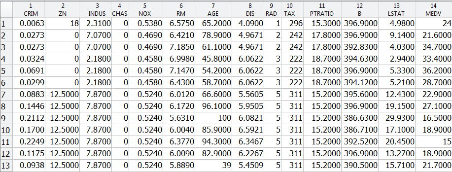
In this example we will explore a regression problem using the Boston House Prices dataset available from the UCI Machine Learning Repository.
filename = 'housing.txt';
urlwrite('http://archive.ics.uci.edu/ml/machine-learning-databases/housing/housing.data',filename);
inputNames = {'CRIM','ZN','INDUS','CHAS','NOX','RM','AGE','DIS','RAD','TAX','PTRATIO','B','LSTAT'};
outputNames = {'MEDV'};
housingAttributes = [inputNames,outputNames];
Once the file is saved, you can import data into MATLAB as a table using the Import Tool with default options. Alternatively you can use the following code which can be auto generated from the Import Tool:
formatSpec = '%8f%7f%8f%3f%8f%8f%7f%8f%4f%7f%7f%7f%7f%f%[^\n\r]';
fileID = fopen(filename,'r');
dataArray = textscan(fileID, formatSpec, 'Delimiter', '', 'WhiteSpace', '',  'ReturnOnError', false);
fclose(fileID);
housing = table(dataArray{1:end-1}, 'VariableNames', {'VarName1','VarName2','VarName3','VarName4','VarName5','VarName6','VarName7','VarName8','VarName9',
'VarName10','VarName11','VarName12','VarName13','VarName14'});

% Delete the file and clear temporary variables
clearvars filename formatSpec fileID dataArray ans;
delete housing.txt
housing.Properties.VariableNames = housingAttributes;
X = housing{:,inputNames};
y = housing{:,outputNames};
rng(5); % For reproducibility

% Set aside 90% of the data for training
cv = cvpartition(height(housing),'holdout',0.1);

t = RegressionTree.template('MinLeaf',5);
mdl = fitensemble(X(cv.training,:),y(cv.training,:),'LSBoost',500,t,...
    'PredictorNames',inputNames,'ResponseName',outputNames{1},'LearnRate',0.01);

L = loss(mdl,X(cv.test,:),y(cv.test),'mode','ensemble');
fprintf('Mean-square testing error = %f\n',L);
Mean-square testing error = 7.056746
figure(1);
% plot([y(cv.training), predict(mdl,X(cv.training,:))],'LineWidth',2);
plot(y(cv.training),'b','LineWidth',2), hold on
plot(predict(mdl,X(cv.training,:)),'r.-','LineWidth',1,'MarkerSize',15)

% Observe first hundred points, pan to view more
xlim([0 100])
legend({'Actual','Predicted'})
xlabel('Training Data point');
ylabel('Median house price');

Plot the predictors sorted on importance.
[predictorImportance,sortedIndex] = sort(mdl.predictorImportance);
figure(2);
barh(predictorImportance)
set(gca,'ytickLabel',inputNames(sortedIndex))
xlabel('Predictor Importance')

figure(3);
trainingLoss = resubLoss(mdl,'mode','cumulative');

testLoss = loss(mdl,X(cv.test,:),y(cv.test),'mode','cumulative');
plot(trainingLoss), hold on
plot(testLoss,'r')
legend({'Training Set Loss','Test Set Loss'})
xlabel('Number of trees');
ylabel('Mean Squared Error');
set(gcf,'Position',[249 634 1009 420])
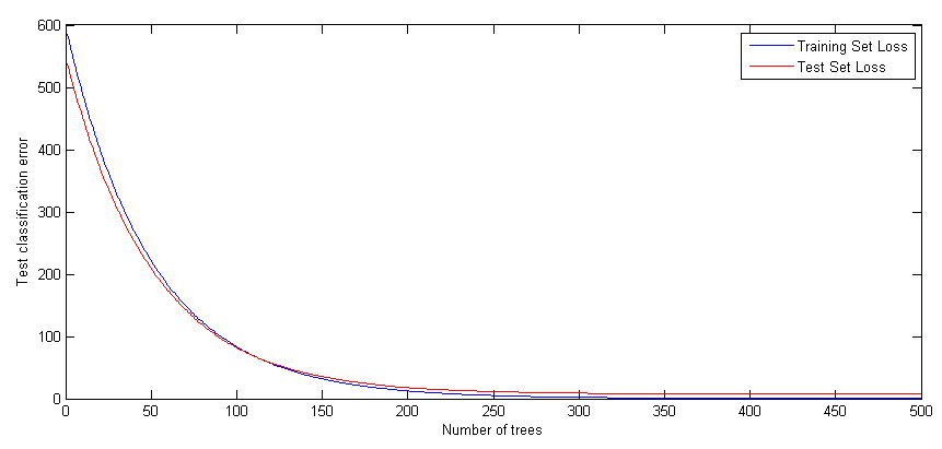
We may not need all 500 trees to get the full accuracy for the model. We can regularize the weights and shrink based on a regularization parameter
% Try two different regularization parameter values for lasso
mdl = regularize(mdl,'lambda',[0.001 0.1]);
disp('Number of Trees:')
disp(sum(mdl.Regularization.TrainedWeights > 0))
Number of Trees:
   194   128
Shrink the ensemble using Lambda = 0.1
mdl = shrink(mdl,'weightcolumn',2);

disp('Number of Trees trained after shrinkage')
disp(mdl.NTrained)
Number of Trees trained after shrinkage
   128
When datasets are large, using a fewer number of trees and fewer predictors based on predictor importance will result in fast computation and accurate results.
Example from scikit-learn.org
License: BSD clause
You can also select a web site from the following list
Americas
- América Latina (Español)
- Canada (English)
- United States (English)
Europe
- Belgium (English)
- Denmark (English)
- Deutschland (Deutsch)
- España (Español)
- Finland (English)
- France (Français)
- Ireland (English)
- Italia (Italiano)
- Luxembourg (English)
- Netherlands (English)
- Norway (English)
- Österreich (Deutsch)
- Portugal (English)
- Sweden (English)
- Switzerland
- United Kingdom (English)
Asia Pacific
- Australia (English)
- India (English)
- New Zealand (English)
- 中国
- 日本Japanese (日本語)
- 한국Korean (한국어)