Creating seamless loop animations by zooming in
This year's MATLAB Shorts Mini Hack contest has kicked off, and there are already lots of interesting entries. The contest features creating a 96-frame, 4-second animation, which is looped 3 times to compose a 12-second short movie. There is an option to add audio to enhance the animation, and it's restricted to a an upper limit of 2,000 characters to promote efficient coding.
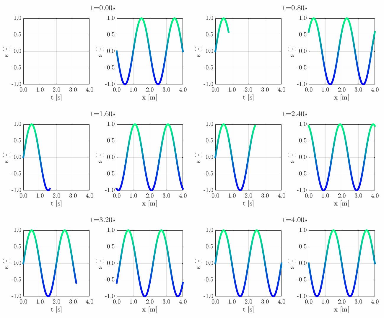
Many of the contestants have already realized the potential for creating a seamless loop, which provides a smooth transition and avoids any discontinuities when the animation is repeated. There are several ways to achieve this. An efficient method for example is utilizing sinusoidal functions, which are periodic, meaning that they repeat themselves over time:
An intuitive example of a seamless loop is @Edgar Guevara's EKG pulse entry, which features an electrocardiogram signal on an oscilloscope. The animation is perfectly matched by the audio, as explained in their post.
Another, rather sophisticated approach is featured in @Tim's Moonrun animation in last year's contest. This seamless loop is achieved by cleverly manipulating the camera position and target over a periodic spatial domain, producing this stunning result:
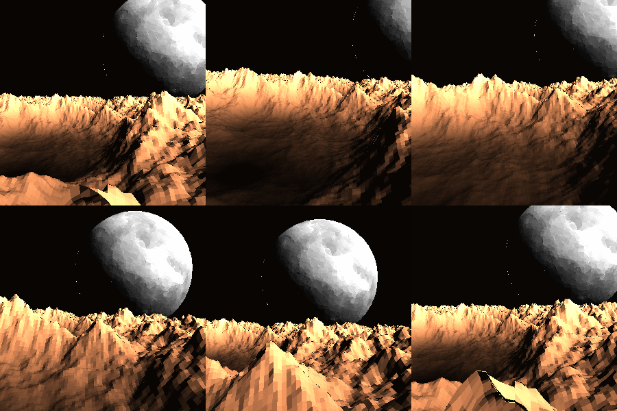
This essentially tells us that for a seamless loop in the spatial domain, the first frame must match the last frame (with a single timestep difference to be more precise, more on that later). But surely this cannot be achieved by zooming in, unless you are simulating a fractal. Well, there are always workarounds.
One way to achieve this is by zooming into a section that contains the first frame of the animation. This is featured in my Winter Loop entry. This is a remix of @Oliver Jaros's Winter entry, which was selected as a one of the weekly winners in the nature & space category for Week 1. The code was modified to lower the character count, but all credits for the original idea and graphics go to them. I also drew inspiration from one of my favourite games of all time, Super Mario 64. Oliver's animation reminded me of the Cool, Cool Mountain level of the game. In the game, you can enter various levels by jumping into paintings serving as portals.
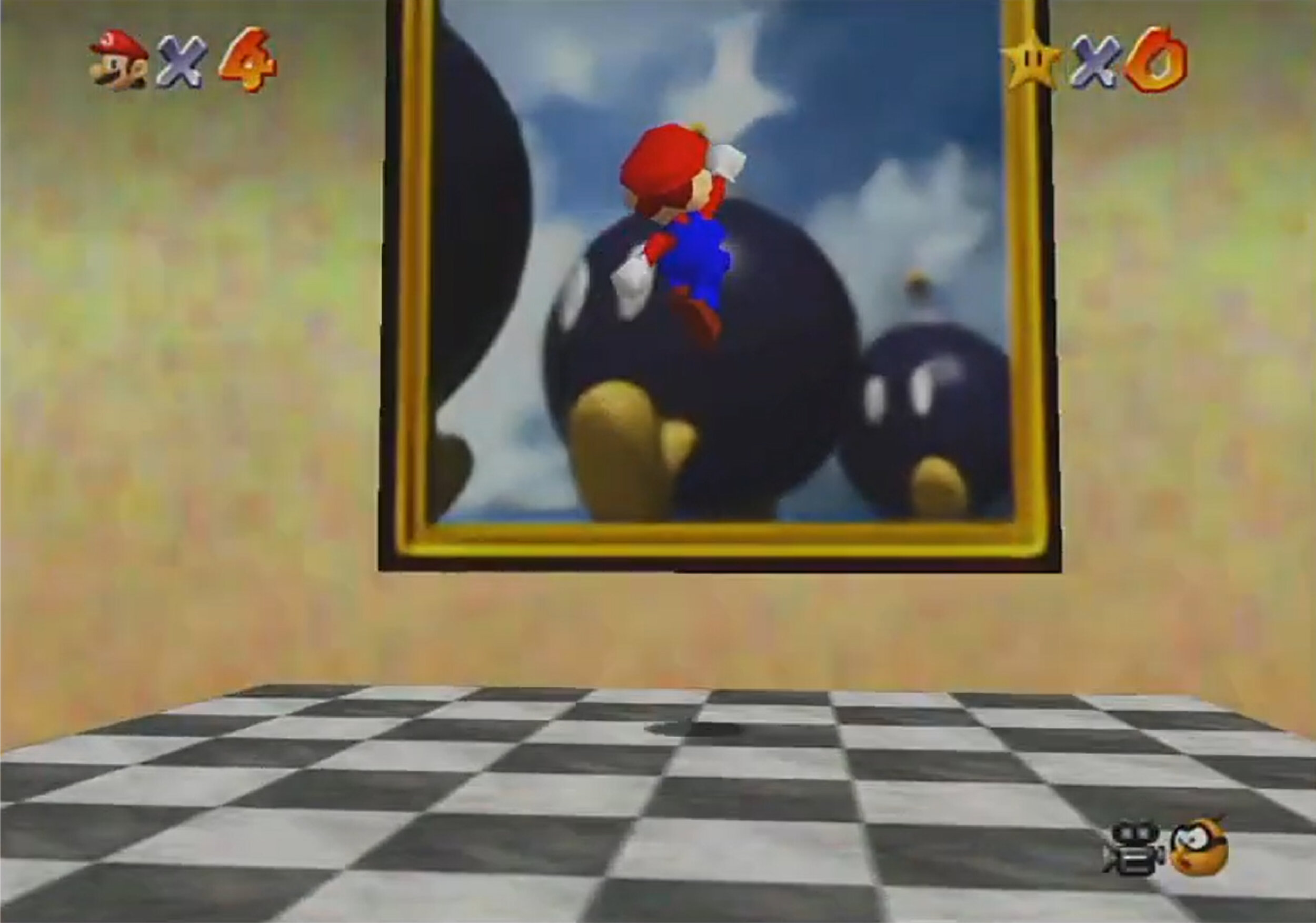
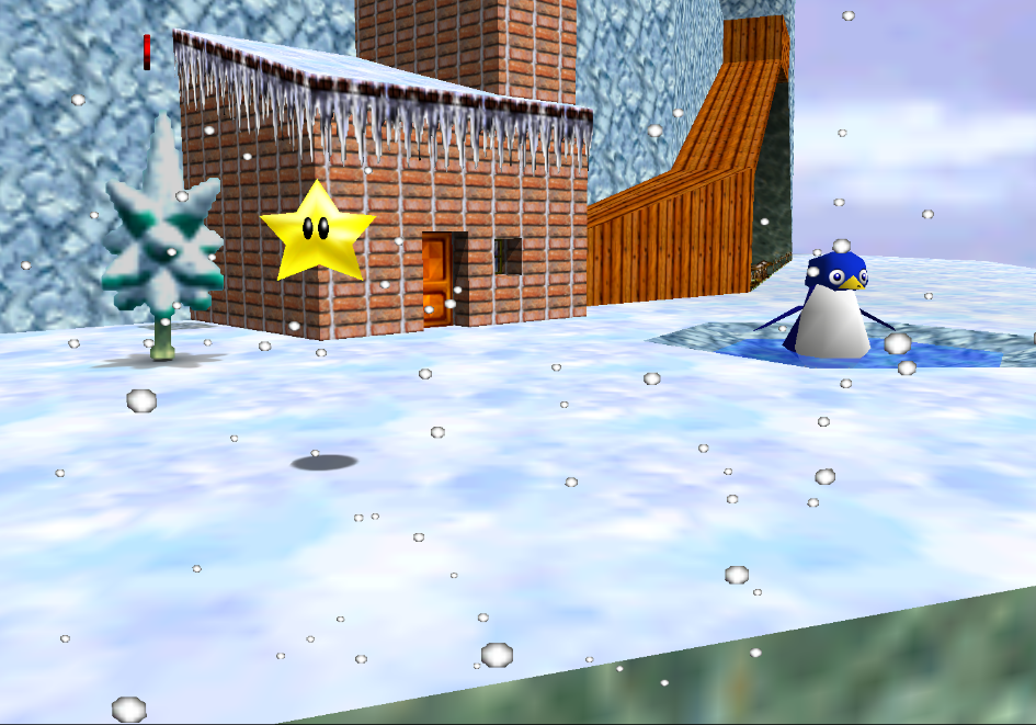
This inspired the idea of zooming into a rectangular photograph frame containing the first frame of the animation to facilitate restarting the loop. One could argue that it would probably take a crazy person to have a photo of their house framed inside their own house. Well, in this economy and with the current house prices, I don't think this scenario is too far-fetched:
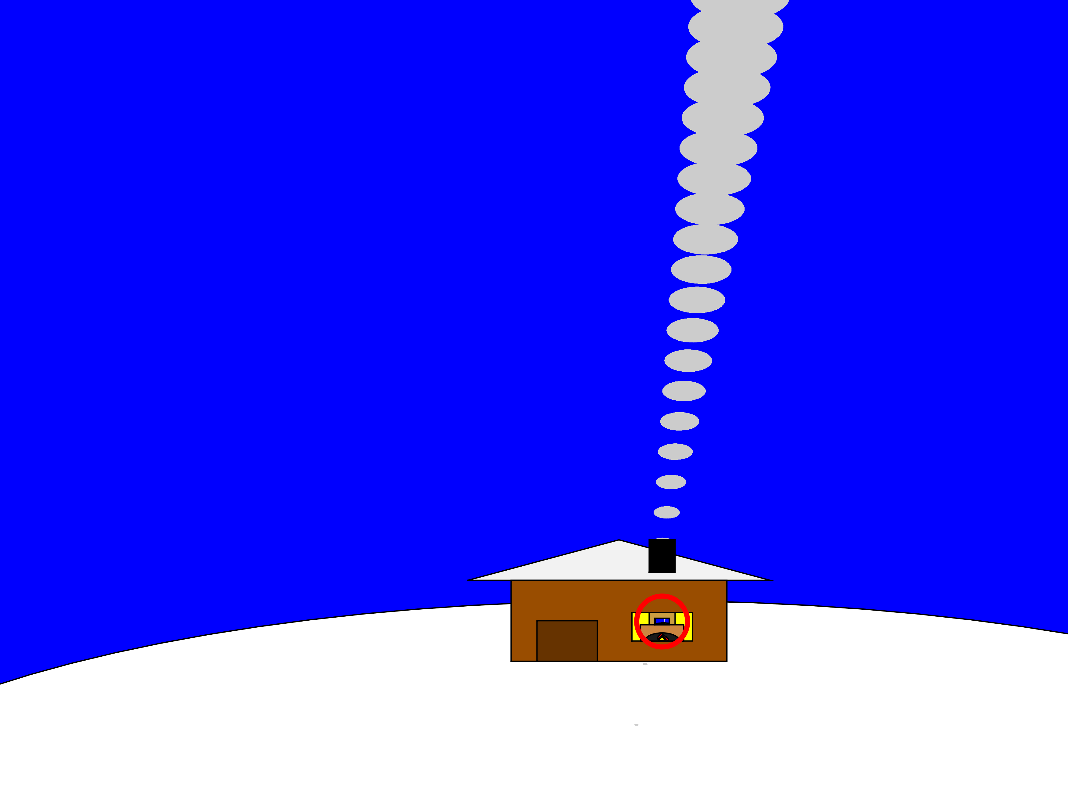
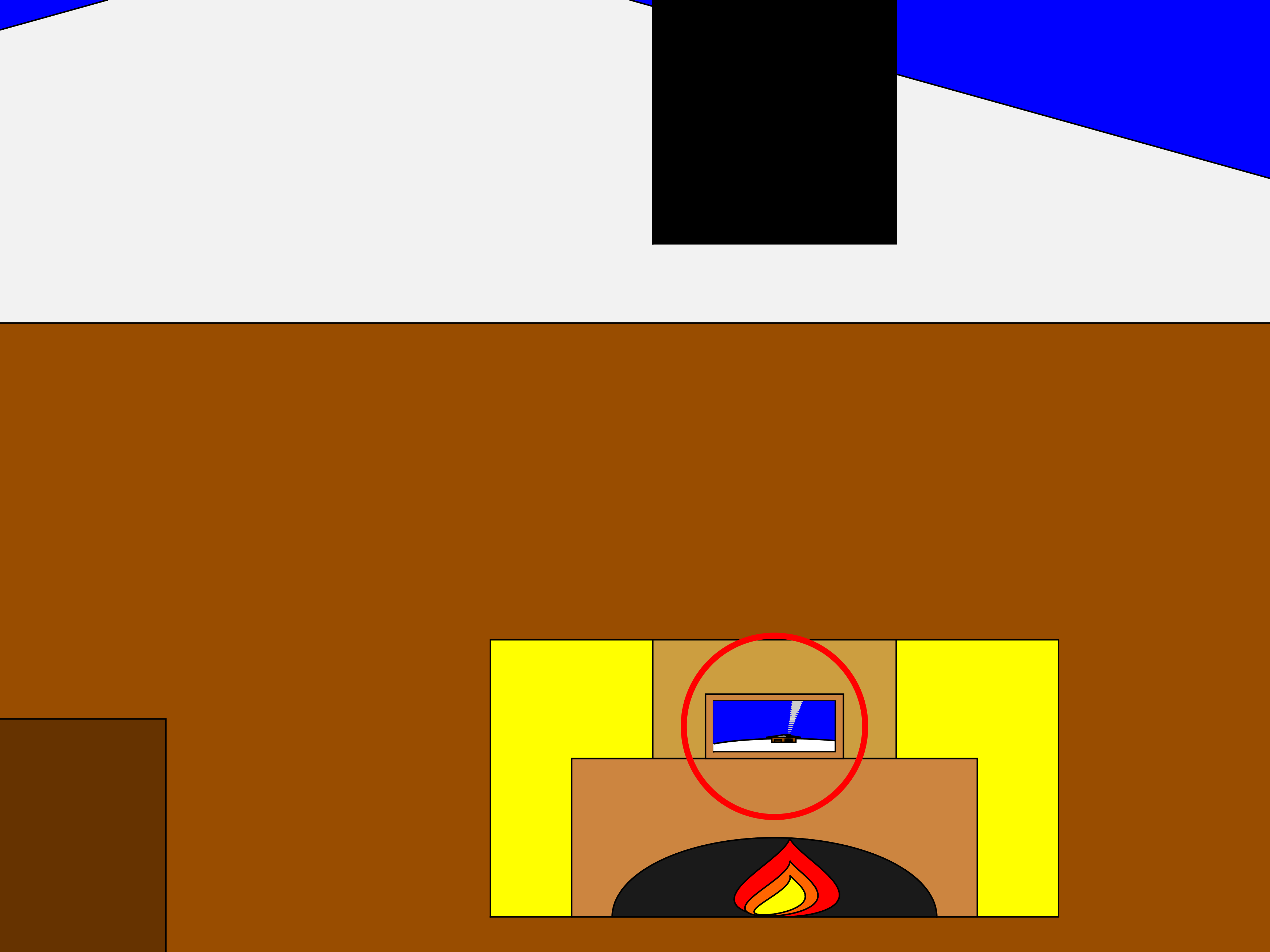
The implementation for this in 2-D is rather simple. Essentially, a second axes is used as the photograph. This is an efficient way of neatly updating the graphics while zooming in. The way this was implemented is explained in the following code snippet, which is a slight modification of the code in the entry:
m = 96; % Number of frames
% Axes limits for the first frame
xm = [xm1,xm2];
ym = [ym1,ym2];
% Axes limits for the last frame (photograph frame edges)
xf = [xf1,xf2];
yf = [yf1,yf2];
% Zoom-in vectors
x1 = linspace(xm(1),xf(1),m+1); % Axes left edge to left photo frame edge
x2 = linspace(xm(2),xf(2),m+1); % Axes right edge to right photo frame edge
y1 = linspace(ym(1),yf(1),m+1); % Axes bottom edge to bottom photo frame edge
y2 = linspace(ym(2),yf(2),m+1); % Axes top edge to top photo frame edge
if f==1
axis([x1(f),x2(f),y1(f),y2(f)]); % Set main axes limits
ax2 = copyobj(gca,gcf); % Create axes for the photo frame containing the first frame graphics objects
end
axis([x1(f+1),x2(f+1),y1(f+1),y2(f+1)]); % Zoom in main axes
lims = axis; % Main axes updated limits
pos = get(gca,'Position'); % Main axes position
% This keeps the relative position of the 2 axes constant:
pos = [pos(1)+diff([lims(1),xf(1)])/diff(lims(1:2))*pos(3),...
pos(2)+diff([lims(3),yf(1)])/diff(lims(3:4))*pos(4),...
diff(xf)/diff(lims(1:2))*pos(3),...
diff(yf)/diff(lims(3:4))*pos(4)];
ax2.Position = pos; % Adjust the relative position
Let's break down the code to explain the process:
- m is the total number of frames in the animation, i.e. 96 frames.
- xm & ym are the main axes limits for frame 1.
- xf & yf are the main axes limits for frame 96, corresponding to the photograph frame's edges.
- x1, x2, y1 & y2 are the zoom-in vectors, linearly spaced from the left, right, bottom & top main axes edges to the corresponding photograph edges. You have probably noticed that these contain m+1=97 points, which is 1 more than the total number of frames. This is done so that the first frame of the animation and the contents of the photograph frame are offset by a single timestep, so that there are no overlapping frames when the animation is looped, thus creating a perfect, seamless loop. That means that the first frame of the animation will contain the main axes zoomed-in by a single timestep, while the last frame of the animation (i.e. the zoomed-in photograph frame) will contain the most zoomed-out version of the graphics. This neatly wraps the animation, and displays the full zoomed-out view when the video stops playing.
- The photograph frame axes are created when f==1 (after setting the initial axes limits) by using the immensely useful copyobj function. This one-liner creates axes containing all graphics objects for the first frame.
- Zooming in on the main axes is then achieved by adjusting the limits using axis([x1(f+1),x2(f+1),y1(f+1),y2(f+1)]). The main axes current limits and position are then saved using the variables lims and pos respectively, in order to adjust the position of the photograph frame axes.
- While zooming in, it's important that the relative position of the 2 axes is kept constant. This is achieved by simply adjusting the position of the photograph frame axes at every frame, by calculating their relative ratios using the abovementioned formula. The first 2 arguments correspond to the (normalized) x and y positions of the lower left corner of the axes, while the third and fourth arguments correspond to the (normalized) width and height respectively. While this formula will work for any position of the main axes, it's a good idea to set the position as set(gca,'Position',[0 0 1 1]) for this contest, in order to take full advantage of the whole allocated window for the animation.
- Finally, note that the graphics are updated for the main axes only, and the above process is repeated for each frame until fully zooming into the photograph frame's axes.
Some of the most curious minds might wonder that while this is well and all with using the second axes to simulate the photograph, what happens to the photograph inside the photograph (and so on...)? Well, the beauty of this method is that you can repeat this as many times as necessary (just apply the formula using the current position and limits of the second axes to adjust the position of the third axes and so on). Given the speed of the animation and the very small size of the photograph inside the photograph, it would be very unlikely that you would need more than 3 axes, but the process is always good to know.
This is the final result:
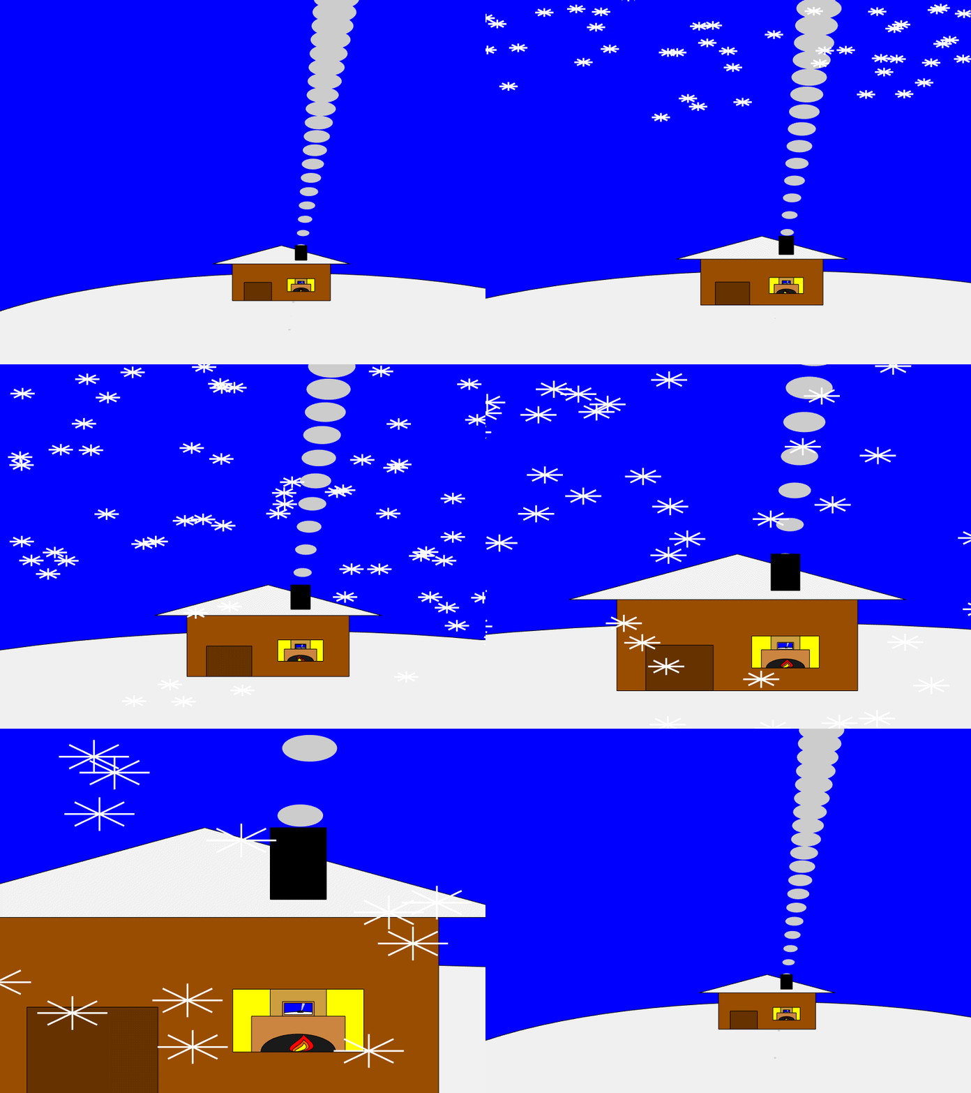
I hope you found these tips useful and I'm looking forward to seeing many creative seamless loop animations in the contest.
3 Comments
Time Descendingawesome article!
That's is the best thing related to
What a great techinical article on creating seamless loop! Thanks for sharing, Vasilis.
Sign in to participate