HDL Neural Network Design for Digital Predistorter
R2026bThis example shows how to design, train, and validate a neural network digital predistorter (NN DPD) that uses segmented spline activations (SSC).The SSC-NN DPD linearizes a power amplifier (PA) driven by a wideband OFDM signal. PAs introduce nonlinear distortion, which causes spectral regrowth and degrades error vector magnitude (EVM). DPD compensates for PA nonlinearity by applying an inverse distortion before the PA. Classical DPD approaches use memory polynomials, which require high polynomial orders and memory depths for wideband signals. NN-based DPD can capture complex nonlinearities with fewer parameters.
This example uses a feedforward neural network with segmented spline activations which are piecewise-linear learnable activation functions that are hardware-friendly and can be implemented as a lookup table with linear interpolation, while providing the expressiveness of smooth nonlinear activations.
In this example, you compare the SSC-NN DPD performance against a classical memory polynomial DPD and verify fixed-point Simulink fidelity before hardware deployment.
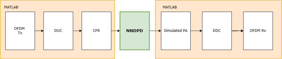
The following diagram shows the end-to-end OFDM signal chain used for DPD validation. The OFDM signal generation, sample rate conversion, and performance evaluation are done in MATLAB(R), while the DPD block highlighted is the device under test (DUT) - a fixed-point Simulink(R) subsystem targeted for HDL code generation.
Signal Generation
Generate an OFDM waveform, upsample with digital upconversion (DUC), and apply crest factor reduction (CFR).
ofdmCfg = getOFDMConfig();

rng(123);
numTxFrames = 1;
radioSampleRate = 122.88e6;

% Generate transmit waveform
txBits = randi([0 1], ofdmCfg.bitsPerFrame, 1);
txWaveformTrain = customOFDMTx(txBits, ofdmCfg);
matTxOut = txWaveformTrain;

% Upsample to radio sample rate
txWaveformTrain = digitalUpconvert(txWaveformTrain, ...
    radioSampleRate/ofdmCfg.ofdmSampleRate, ofdmCfg);

% Measure PAPR and determine CFR threshold
paprTarget = 8; % dB
refImpedance = 1;
pm = powermeter(Measurement="All", ...
    WindowLength=round(radioSampleRate*10e-3), ...
    ReferenceLoad=refImpedance, PowerUnits="dBm");
[avgpwr,~,~] = pm(txWaveformTrain);

avgpwrOFDM = avgpwr(end);
peakInstPow = avgpwrOFDM + paprTarget;
peakInstMag = db2mag(peakInstPow - 30);

% Apply CFR and scale. The 0.875 factor reserves 12.5% headroom below
% full-scale to prevent DAC clipping from residual peaks after CFR.
postCfrScale = 0.875 / peakInstMag;
txWaveformTrain = cfrClip(txWaveformTrain, peakInstMag) * postCfrScale;
scalingFactor = 1/std(txWaveformTrain);
Generate a separate test waveform for evaluation.
txBits = randi([0 1], ofdmCfg.bitsPerFrame, 1);
[txWaveformTest, txDataSymsTest] = customOFDMTx(txBits, ofdmCfg);
[txWaveformTest, filterCoeffs] = digitalUpconvert(txWaveformTest, ...
    radioSampleRate/ofdmCfg.ofdmSampleRate, ofdmCfg);
txWaveformTest = cfrClip(txWaveformTest, peakInstMag) * postCfrScale;
Generate a separate test waveform for validation.
txBits = randi([0 1], ofdmCfg.bitsPerFrame, 1);
[txWaveformVal, txDataSymsVal] = customOFDMTx(txBits, ofdmCfg);
[txWaveformVal, ~] = digitalUpconvert(txWaveformVal, ...
    radioSampleRate/ofdmCfg.ofdmSampleRate, ofdmCfg);
txWaveformVal = cfrClip(txWaveformVal, peakInstMag) * postCfrScale;
PA Behavioral Model
This example uses a neural network trained on data captured from a real PA using an NI VST to model the PA behavior. The trained PA model resides in |paModelNN.mat|. This approach provides a realistic nonlinear model without requiring hardware-in-the-loop (HIL). For details on the PA modeling methodology and training procedure, see Power Amplifier Modeling Using Neural Networks.
% Input backoff to avoid hard saturation
IBO = 8.2; % dB
pmPapr = powermeter(...
    Measurement="Peak-to-average power ratio", ...
    WindowLength=round(radioSampleRate*10e-3), ...
    ReferenceLoad=refImpedance, ...
    PowerUnits="dBm");

paprOFDM = pmPapr(txWaveformTrain);
paprOFDM = paprOFDM(end);

disp("OFDM Tx Waveform PAPR: " + num2str(paprOFDM,4) + "dBm");
OFDM Tx Waveform PAPR: 8.008dBm
if paprOFDM >= IBO
    warning("OFDM signal PAPR is greater than the PA back-off and will saturate")
end
% PA observation without DPD
paObsNoDpd = paObservationPath(txWaveformTest, IBO, refImpedance, radioSampleRate);
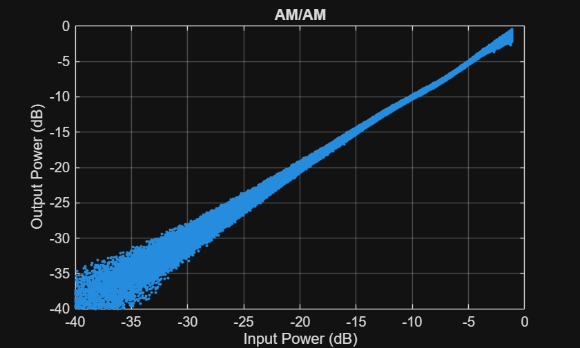
Visualize PA AM/AM characteristics.
helperPANNPlotSpecAnAMAM(txWaveformTest, paObsNoDpd);
SSC-NN DPD Architecture
This example uses the SSC neural network proposed by Vaicaitis and Dooley [1]. The SSC replaces standard activation functions (tanh, ReLU) with piecewise-linear spline segments whose coefficient values are learnable parameters. This design choice reflects hardware implementation constraints.
Low-latency arithmetic - SSC evaluation requires only multiply, add, and subtract. Standard sigmoid activations (
tanh) require iterative algorithms (CORDIC-like), which have several times higher latency than simple arithmetic.Bit-shift segment indexing - Choosing the number of spline segments as a power of two reduces the division operation for locating the active segment to a bit-shift, eliminating the need for a divider or multiplier for indexing.
Fewer active coefficients -
Although total coefficient storage increases with spline length, inference accesses only two coefficients per neuron corresponding to the left and right boundaries of the active segment. The 9-neuron SSC network achieves better normalized mean-square error (NMSE), adjacent channel power ratio (ACPR), and error vector magnitude (EVM) than comparable RVTDNN and ARVTDNN models while using fewer active coefficients.No bias or envelope terms needed - Spline coefficients implicitly capture bias, and SSC flexibility models envelope-dependent behavior without requiring explicit envelope inputs.
The DPD network has the following components:
Input preprocessor - Forms memory taps of depth 2 and separates real and imaginary parts, producing a 4-element input vector per sample.
Fully connected layer - Maps 4 inputs to 9 neurons (hidden layer).
SSC activation layer - Assigns each neuron a segmented spline with 9 coefficients. The spline is piecewise linear between adjacent coefficients, and the coefficient values are learnable parameters.
Output fully connected layer - Maps 9 inputs to 2 outputs, real and imaginary parts of the predistorted signal.
The SSC layer is hardware-friendly because it reduces to a lookup table with linear interpolation - no multipliers beyond the interpolation weight.
memDepth = 2;
inputLayerDim = 2 * memDepth;
numNeurons = 9;
% numSplineCoeffs must be 2^N + 1 (e.g., 3, 5, 9, 17, 33) so that
% deltaInverse is a power of 2, enabling pure bit-shift indexing in HDL.
numSplineCoeffs = 9;
Display the network architecture.
dpdNet = dlnetwork;

tempNet = ([featureInputLayer(inputLayerDim,"Name","input")
    fullyConnectedLayer(numNeurons,"Name","linear1","BiasLearnRateFactor",0)
    SSCLayer(numSplineCoeffs)]);

tempNet(3).Name = "ssc1";

dpdNet = addLayers(dpdNet,tempNet);

tempNet = selectLayer([memDepth 2*memDepth]);
tempNet.Name = "iqInput";
dpdNet = addLayers(dpdNet,tempNet);

tempNet = [
    concatenationLayer(1,2,"Name","concat")
    fullyConnectedLayer(2,"Name","linearOutput")];
dpdNet = addLayers(dpdNet,tempNet);

dpdNet = connectLayers(dpdNet,"ssc1","concat/in1");
dpdNet = connectLayers(dpdNet,"iqInput","concat/in2");
dpdNet = connectLayers(dpdNet,"input","iqInput");

dpdNet = initialize(dpdNet);
analyzeNetwork(dpdNet);
DPD Training
Train the DPD using the indirect learning architecture (ILA) [1]. The network learns the inverse PA model: it takes the PA output (post-observation path) as input and targets the original clean PA input. Once the network converges, copy the trained coefficients directly into the predistorter block. Repeat this process over multiple ILA iterations until performance saturates.
ILA is chosen over Direct Learning Architecture (DLA) because it does not require a differentiable PA model for back propagation — the network simply learns a regression from distorted to clean samples. This pairs well with the SSC activation, whose piecewise-linear segments yield simple constant gradients (the slope of each active segment), making training stable and fast.
Set trainNow = true to retrain the network. By default, pre-trained weights are loaded from dpdNetTrained.mat.
trainNow =false; if trainNow % Define network structure % https://www.mdpi.com/1424-8220/24/6/1829 % https://ieeexplore.ieee.org/document/9916226 nnDPDinputPreproc = dpdPreprocessor(memDepth,1); % Validation data paObsVal = paObservationPath(txWaveformVal, IBO, refImpedance, radioSampleRate); dpdNetInputVal = nnDPDinputPreproc(paObsVal*scalingFactor); reset(nnDPDinputPreproc); dpdNetTargetVal = [real(txWaveformVal), imag(txWaveformVal)]*scalingFactor; % Define training paramaters maxEpochs = 20; miniBatchSize = 1024; iterPerEpoch = floor(size(txWaveformVal, 1)/miniBatchSize); trainingPlots =
"training-progress"; metrics =
[]; verbose =
false; options = trainingOptions('adam', ... MaxEpochs=maxEpochs, ... MiniBatchSize=miniBatchSize, ... InitialLearnRate=4e-4, ... LearnRateDropFactor=0.95, ... LearnRateDropPeriod=5, ... LearnRateSchedule='piecewise', ... Shuffle='every-epoch', ... OutputNetwork='best-validation-loss', ... ValidationData={dpdNetInputVal,dpdNetTargetVal}, ... ValidationFrequency=2*iterPerEpoch, ... ValidationPatience=5, ... InputDataFormats="BC", ... TargetDataFormats="BC", ... ExecutionEnvironment='auto', ... Plots=trainingPlots, ... Metrics = metrics, ... Verbose=verbose, ... VerboseFrequency=2*iterPerEpoch); numILAIterations = 2; for ii = 1:numILAIterations if ii > 1 % Feed txWaveTrain through predistorter trained in the previous % iteration dpdNetInputPreDistortTrain = nnDPDinputPreproc(txWaveformTrain*scalingFactor); reset(nnDPDinputPreproc); nnDpdOut = predict(dpdNet,dpdNetInputPreDistortTrain); txWaveformTrainIter = double(complex(nnDpdOut(:,1),nnDpdOut(:,2)))./ scalingFactor; else txWaveformTrainIter = txWaveformTrain; end paObsTrain = paObservationPath(txWaveformTrainIter, IBO, refImpedance, radioSampleRate); dpdNetInputTrain = nnDPDinputPreproc(paObsTrain*scalingFactor); reset(nnDPDinputPreproc); dpdNetTargetTrain = [real(txWaveformTrainIter), imag(txWaveformTrainIter)]*scalingFactor; dpdNet = trainnet(dpdNetInputTrain,dpdNetTargetTrain,dpdNet,"mse",options); end save("dpdNetTrained","dpdNet"); else load("dpdNetTrained"); end
SSC-NN DPD - MATLAB Inference
Run the trained DPD network on the test waveform in MATLAB.
nnDPDinputPreproc = dpdPreprocessor(memDepth, 1);
dpdNetInputTest = nnDPDinputPreproc(txWaveformTest * scalingFactor);
reset(nnDPDinputPreproc);

nnDpdOut = predict(dpdNet, dpdNetInputTest);

nnDpdOut = double(complex(nnDpdOut(:,1), nnDpdOut(:,2))) ./ scalingFactor;

paObsNNDpd = paObservationPath(nnDpdOut, IBO, refImpedance, radioSampleRate);
SSC-NN DPD - Fixed-Point Simulink Verification
Run the same test waveform through the Simulink NNDPD subsystem to verify that fixed-point quantization does not degrade performance. This validates the HDL-ready model before hardware deployment.
The top-level model streams the test waveform one sample per clock into the NNDPD subsystem, which contains three stages: Pre-Process, SSC Network, and Post-Process. The Pre-Process stage applies the scaling factor, computes delay terms (memory taps based on memory depth), and separates real and imaginary components into a vector input for the network. A valid signal propagates alongside data through the pipeline.
modelName = 'HDLNNDigitalPredistorter';
load_system(modelName)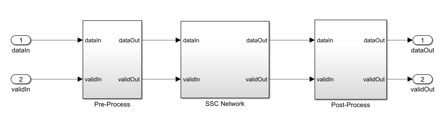
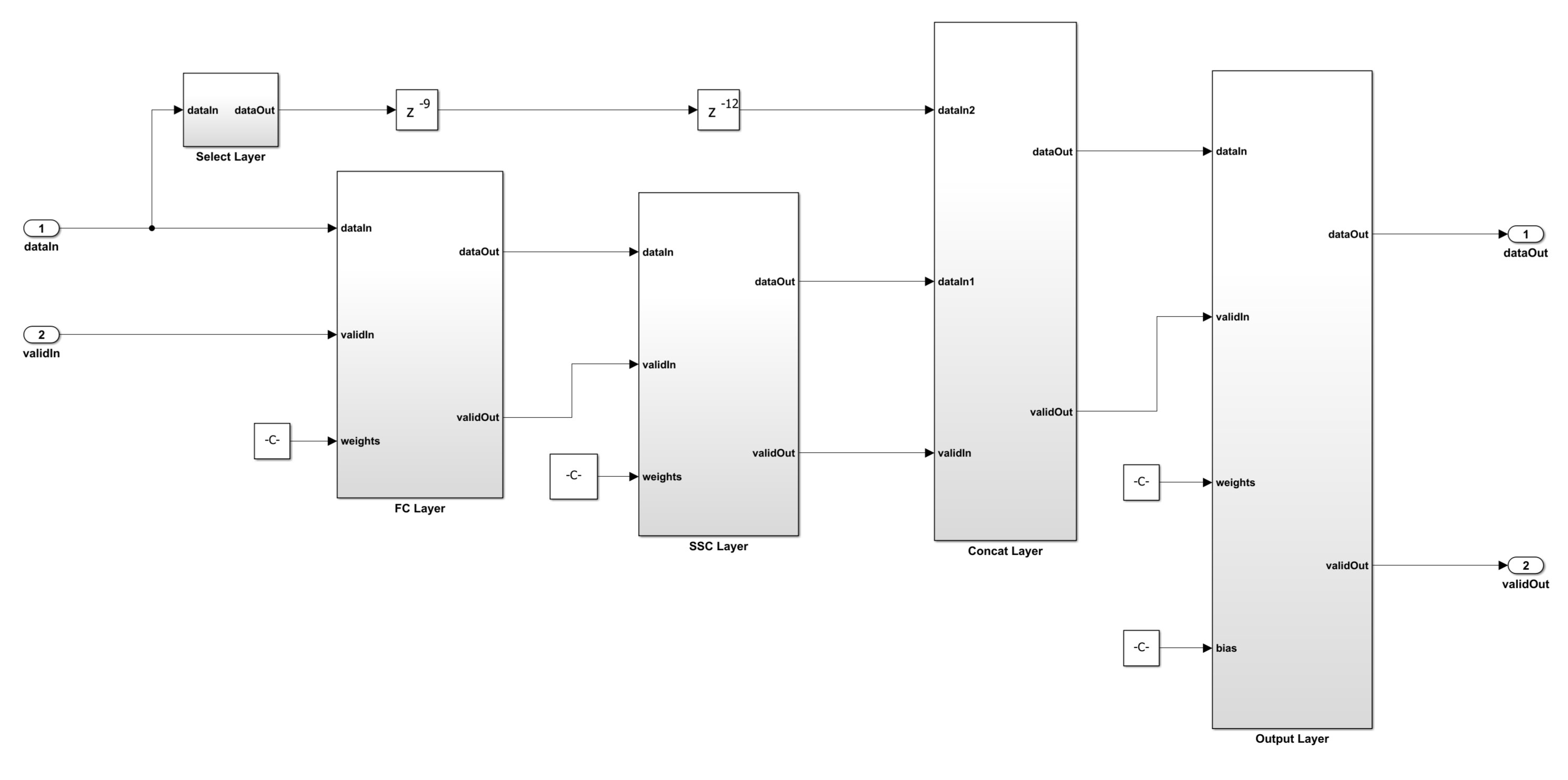
Inside the SSC Network, the signal flows through: a FC Layer (fixed-point multiply-accumulate), an SSC Layer (piecewise-linear spline lookup with learnable coefficient values), a Select Layer that provides the linear I/Q skip connection, a Concat Layer that merges the SSC output with the skip path, and an Output Layer that produces the final 2-element predistorted output. Pipeline delays between stages align the data and valid signals.
numSamples = length(txWaveformTest);
samplesPerCycle = 1;
latency = 49;
stopTime = (numSamples+latency) / ofdmCfg.ofdmSampleRate;

out = sim(modelName);
simpaObsNNDPD = paObservationPath(double(out.nnDpdOut), IBO, refImpedance, radioSampleRate);
simpaObsNNDPD = simpaObsNNDPD(1:length(paObsNNDpd));
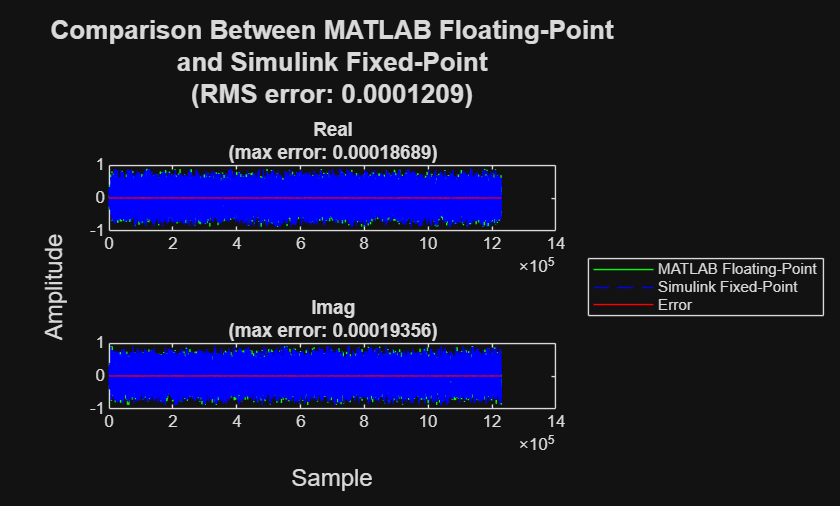
Compare the MATLAB floating-point and Simulink fixed-point DPD outputs to confirm quantization fidelity.
plotSignalComparison(nnDpdOut, double(out.nnDpdOut), ...
    "MATLAB Floating-Point", "Simulink Fixed-Point");
Classical DPD Baseline
Train a classical memory polynomial DPD as a performance baseline. The memory polynomial model captures both the nonlinear and memory effects of the PA by using a set of basis functions formed from delayed input samples raised to various powers. Here, a nonlinear degree of 5 and memory depth of 5 are used, resulting in 25 complex coefficients estimated via least squares. This configuration represents a typical classical DPD implementation and serves as the reference for evaluating the SSC-NN approach in terms of both linearization performance and hardware cost.
paObsTrain = paObservationPath(txWaveformTrain, IBO, refImpedance, radioSampleRate);

estimator = comm.DPDCoefficientEstimator( ...
    DesiredAmplitudeGaindB=0, ...
    PolynomialType="Memory polynomial", ...
    Degree=5, MemoryDepth=5, Algorithm="Least squares");

coef = estimator(txWaveformTrain, paObsTrain);
dpdMem = comm.DPD(PolynomialType="Memory polynomial", Coefficients=coef);

classicalDpdOut = dpdMem(txWaveformTest);
paObsClassDpd = paObservationPath(classicalDpdOut, IBO, refImpedance, radioSampleRate);
Spectral Comparison
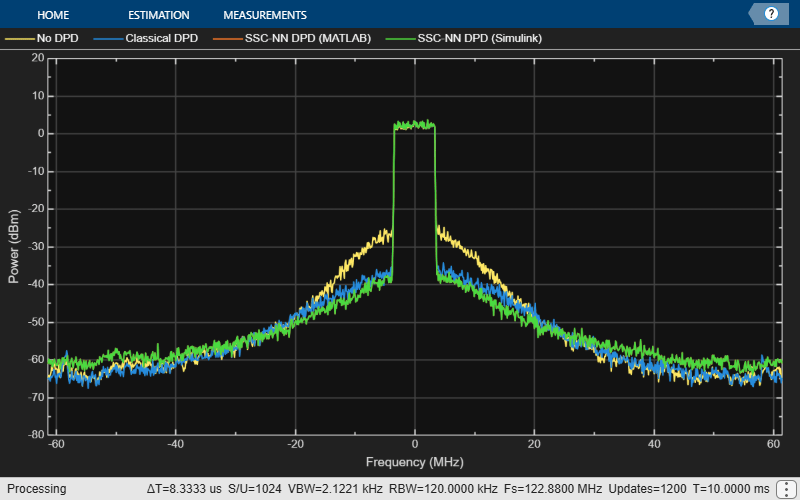
Compare the output spectra of the PA without DPD, with classical memory polynomial DPD (Degree 5, Memory Depth 5), and with SSC-NN DPD (9 neurons, 9 spline segments) in both MATLAB floating-point and Simulink fixed-point.
sa = spectrumAnalyzer;
sa.SpectrumType = "Power";
sa.SampleRate = radioSampleRate;
sa.ReferenceLoad = refImpedance;
sa.ChannelNames = {"No DPD", "Classical DPD", "SSC-NN DPD (MATLAB)", "SSC-NN DPD (Simulink)"};
sa([paObsNoDpd, paObsClassDpd, paObsNNDpd, simpaObsNNDPD]);
sa.ShowLegend = true;
Performance Comparison
Compute ACPR and NMSE for each configuration.
acprNoDPD       = helperACPR(paObsNoDpd, radioSampleRate, ofdmCfg.ofdmSampleRate);
acprClassDPD    = helperACPR(paObsClassDpd, radioSampleRate, ofdmCfg.ofdmSampleRate);
acprNNDPD       = helperACPR(paObsNNDpd, radioSampleRate, ofdmCfg.ofdmSampleRate);
acprSimNNDPD    = helperACPR(simpaObsNNDPD, radioSampleRate, ofdmCfg.ofdmSampleRate);

nmseNoDPD    = 10*log10(sum(abs(paObsNoDpd - txWaveformTest).^2) / sum(abs(txWaveformTest).^2));
nmseClassDPD = 10*log10(sum(abs(paObsClassDpd - txWaveformTest).^2) / sum(abs(txWaveformTest).^2));
nmseNNDPD    = 10*log10(sum(abs(paObsNNDpd - txWaveformTest).^2) / sum(abs(txWaveformTest).^2));
nmseSimNNDPD = 10*log10(sum(abs(simpaObsNNDPD - txWaveformTest).^2) / sum(abs(txWaveformTest).^2));

perfTable = table( ...
    [acprNoDPD; acprClassDPD; acprNNDPD; acprSimNNDPD], ...
    [nmseNoDPD; nmseClassDPD; nmseNNDPD; nmseSimNNDPD], ...
    VariableNames=["ACPR_dB", "NMSE_dB"], ...
    RowNames=["No DPD", "Classical DPD", "SSC-NN DPD (MATLAB)", "SSC-NN DPD (Simulink)"]);
disp(perfTable)
                             ACPR_dB    NMSE_dB
                             _______    _______

    No DPD                   -30.772    -22.825
    Classical DPD            -39.159    -33.251
    SSC-NN DPD (MATLAB)        -40.9      -36.2
    SSC-NN DPD (Simulink)    -40.901    -36.197
EVM and Constellation Analysis
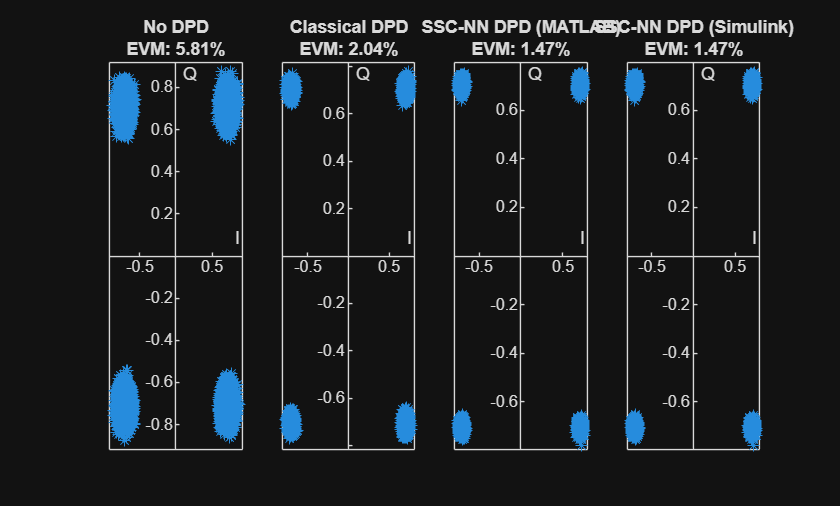
Demodulate the received signal and compute EVM for each DPD configuration.
rxSourceOpts = ["No DPD", "Classical DPD", "SSC-NN DPD (MATLAB)", "SSC-NN DPD (Simulink)"];
paObsAll = {paObsNoDpd, paObsClassDpd, paObsNNDpd, simpaObsNNDPD};

figure;
tiledlayout(1, numel(rxSourceOpts));

for ii = 1:numel(rxSourceOpts)
    rxWaveform = digitalDownconvert(paObsAll{ii}, 16, ofdmCfg);
    refScale = rms(matTxOut) / rms(rxWaveform);
    rxWaveform = refScale * rxWaveform ./ max(abs(rxWaveform));

    [~, rxDataSymsEq] = customOFDMRx(rxWaveform, 0, ofdmCfg);

    evm = comm.EVM;
    rmsEVM(ii) = evm(txDataSymsTest, rxDataSymsEq);

    nexttile;
    plotConstellation(rxDataSymsEq, ...
        rxSourceOpts(ii) + newline + "EVM: " + num2str(rmsEVM(ii), '%.2f') + "%");
end
HDL Code Generation and Synthesis Results
To check and generate HDL for this example, you must have HDL Code(TM). Use the |makehdl| and |makehdltb| commands to generate the HDL code and test bench for the NNDPD subsystem.
When you synthesize the NNDPD subsystem on AMD Zynq(TM) UltraScale+(TM) RFSoC ZCU111 evaluation kit, the frequency obtained after post map is about 509 MHz. This table shows the post map resource utilization results for a 16-bit complex input.
F = table(...
    categorical({'CLB LUTs'; 'CLB Registers';'DSP'}), ...
    categorical({'11777'; '16822'; '58'}), ...
    categorical({'425280'; '850560'; '4272'}), ...
    categorical({'1.62'; '1.36'; '1.66'}), ...
    'VariableNames', ...
    {'Resources','Utilized','Available','Utilization (%)'});
disp(F);
      Resources      Utilized    Available    Utilization (%)
    _____________    ________    _________    _______________

    CLB LUTs          11777       425280           1.62
    CLB Registers     16822       850560           1.36
    DSP               58          4272             1.66
Summary
This example demonstrated a segmented spline curve neural network for digital predistortion, from algorithm design through HDL-ready implementation. The network is trained using indirect learning architecture with a simulated PA model derived from real NI VST measurements. The following table summarizes the performance and resource comparison.
T = table( ...
    categorical({'No DPD'; 'Classical DPD (Degree-3/Depth-3)'; 'Classical DPD (Degree-5/Depth-5)'; 'SSC-NN DPD (n=9, s=9)'}), ...
    [acprNoDPD; -36.631; acprClassDPD; acprSimNNDPD], ...
    categorical({'0'; '50'; '144'; '58'}), ...
    'VariableNames', {'Configuration', 'ACPR (dB)', 'Real Multipliers'});
disp(T);
             Configuration              ACPR (dB)    Real Multipliers
    ________________________________    _________    ________________

    No DPD                               -30.772           0
    Classical DPD (Degree-3/Depth-3)     -36.631           50
    Classical DPD (Degree-5/Depth-5)     -39.159           144
    SSC-NN DPD (n=9, s=9)                -40.901           58
At a comparable multiplier count (~58 vs ~50), the SSC-NN DPD achieves 4 dB better ACPR than the classical Degree-3 memory polynomial. To match the SSC-NN performance, the classical approach requires Degree-5 with nearly 3x the multipliers. The fixed-point Simulink simulation matches MATLAB floating-point results within ~0.5 dB ACPR, confirming quantization fidelity before HDL code generation. The design processes one sample per clock at 509 MHz, making it suitable for high bandwidth applications up to 500 MSPS.
References
[1] A. Vaicaitis and J. Dooley, "Segmented Spline Curve Neural Network for Low Latency Digital Predistortion of RF Power Amplifiers," IEEE Trans. Microw. Theory Techn., vol. 70, no. 11, pp. 4910–4915, Nov. 2022.

