Wavelet Scattering Invariance Scale and Oversampling

Open Live Script

This example shows how changing the invariance scale and oversampling factor affects the output of the wavelet scattering transform.

Invariance Scale

The InvarianceScale property of a wavelet time scattering network sets the time scale of the scaling (lowpass) filter. Create a wavelet scattering network with a signal length of 10,000 and invariance scale of 500. Obtain the filter bank.

sigLength = 1e4;
sf = waveletScattering('SignalLength',sigLength,'InvarianceScale',500);
[fb,f] = filterbank(sf);

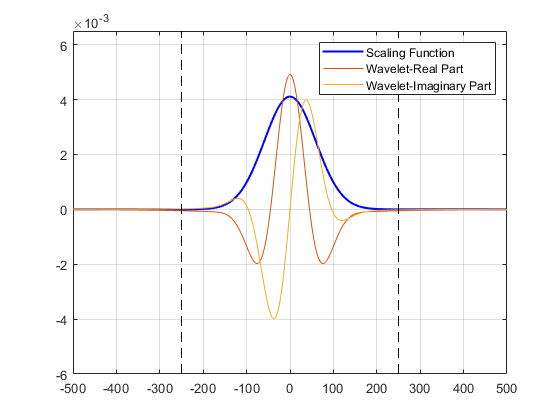
Use the helper function helperPlotScalingWavelet to plot the scaling filter in time along with the real and imaginary parts of the coarsest-scale wavelet from the first filter bank. The source code for helperPlotScalingWavelet is listed in the appendix. The supports of the scaling filter and wavelet are essentially the size of the invariance scale.

helperPlotScalingWavelet(fb,f,500)

Generate a random signal and use featureMatrix to obtain the scattering feature matrix for the signal and scattering network.

x = randn(1,sigLength);
smat = featureMatrix(sf,x);
whos smat

  Name        Size            Bytes  Class     Attributes

  smat      102x79            64464  double

Each row of the feature matrix is a vector which has been convolved (filtered) with the lowpass filter (after other wavelet filtering). The second dimension of the feature matrix is the time resolution. The output of the filtering is downsampled as much as possible without aliasing, what is called "critically downsampling". The amount of downsampling depends on the bandwidth of the filter. The bigger the invariance scale, the larger the time support of the lowpass (scaling) function and accordingly the more we can downsample.

Obtain the scattering transform of the signal.

[S,~] = scatteringTransform(sf,x);
S{2}

ans=41×4 table
       signals        path      bandwidth    resolution
    _____________    _______    _________    __________

    {79×1 double}    0     1    0.0084478        -7    
    {79×1 double}    0     2    0.0084478        -7    
    {79×1 double}    0     3    0.0084478        -7    
    {79×1 double}    0     4    0.0084478        -7    
    {79×1 double}    0     5    0.0084478        -7    
    {79×1 double}    0     6    0.0084478        -7    
    {79×1 double}    0     7    0.0084478        -7    
    {79×1 double}    0     8    0.0084478        -7    
    {79×1 double}    0     9    0.0084478        -7    
    {79×1 double}    0    10    0.0084478        -7    
    {79×1 double}    0    11    0.0084478        -7    
    {79×1 double}    0    12    0.0084478        -7    
    {79×1 double}    0    13    0.0084478        -7    
    {79×1 double}    0    14    0.0084478        -7    
    {79×1 double}    0    15    0.0084478        -7    
    {79×1 double}    0    16    0.0084478        -7    
      ⋮

The scattering coefficient vectors, signals, have length 79, and the resolution is -7. This means that we expect approximately $1 0^{4} / 2^{7}$ coefficients in each vector.

Create a wavelet scattering network with an invariance scale of 200. Obtain the scattering transform of the signal. Because the invariance scale is smaller, the bandwidth of the scaling filter increases and we cannot downsample as much without aliasing. Therefore, the number of scattering coefficients increases.

sf = waveletScattering('SignalLength',sigLength,'InvarianceScale',200);
[S,~] = scatteringTransform(sf,x);
S{2}

ans=30×4 table
       signals         path      bandwidth    resolution
    ______________    _______    _________    __________

    {157×1 double}    0     1     0.02112         -6    
    {157×1 double}    0     2     0.02112         -6    
    {157×1 double}    0     3     0.02112         -6    
    {157×1 double}    0     4     0.02112         -6    
    {157×1 double}    0     5     0.02112         -6    
    {157×1 double}    0     6     0.02112         -6    
    {157×1 double}    0     7     0.02112         -6    
    {157×1 double}    0     8     0.02112         -6    
    {157×1 double}    0     9     0.02112         -6    
    {157×1 double}    0    10     0.02112         -6    
    {157×1 double}    0    11     0.02112         -6    
    {157×1 double}    0    12     0.02112         -6    
    {157×1 double}    0    13     0.02112         -6    
    {157×1 double}    0    14     0.02112         -6    
    {157×1 double}    0    15     0.02112         -6    
    {157×1 double}    0    16     0.02112         -6    
      ⋮

Oversampling Factor

Because the invariance scale is such an important hyperparameter for scattering networks (one of the most important for performance), you should set the value based on the problem at hand and not because you want a certain number of coefficients. You can use the OversamplingFactor property for adjusting the number of coefficients for a given InvarianceScale. The OversamplingFactor specifies how much the scattering coefficients are oversampled with respect to the critically downsampled values. The factor is on a $\log_{2}$ scale.

Create a scattering network with an invariance scale of 500, and an OversamplingFactor equal to 1. Obtain the scattering transform of the signal. As expected, the number of scattering paths is greater than in the case where InvarianceScale is 200. By setting OversamplingFactor to 1, the scattering transform returns two times as many coefficients for each scattering path with respect to the critically sampled number. The size of the scattering coefficient vectors returned is equal to the size when the scattering network has an invariance scale of 200 with default critical downsampling.

sf = waveletScattering('SignalLength',sigLength,'InvarianceScale',500,'OversamplingFactor',1);
[S,~] = scatteringTransform(sf,x);
S{2}

ans=41×4 table
       signals         path      bandwidth    resolution
    ______________    _______    _________    __________

    {157×1 double}    0     1    0.0084478        -6    
    {157×1 double}    0     2    0.0084478        -6    
    {157×1 double}    0     3    0.0084478        -6    
    {157×1 double}    0     4    0.0084478        -6    
    {157×1 double}    0     5    0.0084478        -6    
    {157×1 double}    0     6    0.0084478        -6    
    {157×1 double}    0     7    0.0084478        -6    
    {157×1 double}    0     8    0.0084478        -6    
    {157×1 double}    0     9    0.0084478        -6    
    {157×1 double}    0    10    0.0084478        -6    
    {157×1 double}    0    11    0.0084478        -6    
    {157×1 double}    0    12    0.0084478        -6    
    {157×1 double}    0    13    0.0084478        -6    
    {157×1 double}    0    14    0.0084478        -6    
    {157×1 double}    0    15    0.0084478        -6    
    {157×1 double}    0    16    0.0084478        -6    
      ⋮

Appendix

function helperPlotScalingWavelet(fb,f,invScale)
% This function is in support of wavelet scattering examples only. It may
% change or be removed in a future release.
fBin = diff(f(1:2));
time = (-1/2:fBin:1/2-fBin)*1e4;
phi = ifftshift(ifft(fb{1}.phift));
psiL1 = ifftshift(ifft(fb{2}.psift(:,end)));
figure
plot(time,phi,'b','LineWidth',1.5)
grid on
hold on
plot(time,real(psiL1));
plot(time,imag(psiL1));
plot([-invScale/2 -invScale/2],[-6e-3 6.5e-3],'k--')
plot([invScale/2 invScale/2],[-6e-3 6.5e-3],'k--')
ylim([-6e-3 6.5e-3])
xlim([-invScale invScale])
legend('Scaling Function','Wavelet-Real Part','Wavelet-Imaginary Part')
end

Wavelet Scattering Invariance Scale and Oversampling

Invariance Scale

Oversampling Factor

Appendix

See Also