Main Content

Least Asymmetric Wavelet and Phase

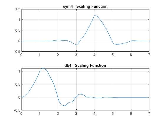
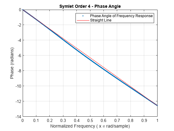
For a given support, the orthogonal wavelet with a phase response that most closely resembles a linear phase filter is called least asymmetric. Symlets are examples of least asymmetric wavelets. They are modified versions of the classic Daubechies db wavelets. In this example you will show that the order 4 symlet has a nearly linear phase response, while the order 4 Daubechies wavelet does not.

First plot the order 4 symlet and order 4 Daubechies scaling functions. While neither is perfectly symmetric, note how much more symmetric the symlet is.

[phi_sym,~,xval_sym]=wavefun('sym4',10);
[phi_db,~,xval_db]=wavefun('db4',10);
subplot(2,1,1)
plot(xval_sym,phi_sym)
title('sym4 - Scaling Function')
grid on
subplot(2,1,2)
plot(xval_db,phi_db)
title('db4 - Scaling Function')
grid on

Generate the filters associated with the order 4 symlet and Daubechies wavelets.

scal_sym = symaux(4,sqrt(2));
scal_db = dbaux(4,sqrt(2));

Compute the frequency response of the scaling synthesis filters.

[h_sym,w_sym] = freqz(scal_sym);
[h_db,w_db] = freqz(scal_db);

To avoid visual discontinuities, unwrap the phase angles of the frequency responses and plot them. Note how well the phase angle of the symlet filter approximates a straight line.

h_sym_u = unwrap(angle(h_sym));
h_db_u = unwrap(angle(h_db));
figure
plot(w_sym/pi,h_sym_u,'.')
hold on
plot(w_sym([1 end])/pi,h_sym_u([1 end]),'r')
grid on
xlabel('Normalized Frequency ( x \pi rad/sample)')
ylabel('Phase (radians)')
legend('Phase Angle of Frequency Response','Straight Line')
title('Symlet Order 4 - Phase Angle')

figure
plot(w_db/pi,h_db_u,'.')
hold on
plot(w_db([1 end])/pi,h_db_u([1 end]),'r')
grid on
xlabel('Normalized Frequency ( x \pi rad/sample)')
ylabel('Phase (radians)')
legend('Phase Angle of Frequency Response','Straight Line')
title('Daubechies Order 4 - Phase Angle')

The sym4 and db4 wavelets are not symmetric, but the biorthogonal wavelet is. Plot the scaling function associated with the bior3.5 wavelet. Compute the frequency response of the synthesis scaling filter for the wavelet and verify that it has linear phase.

[~,~,phi_bior_r,~,xval_bior]=wavefun('bior3.5',10);
figure
plot(xval_bior,phi_bior_r)
title('bior3.5 - Scaling Function')
grid on

[LoD_bior,HiD_bior,LoR_bior,HiR_bior] = wfilters('bior3.5');
[h_bior,w_bior] = freqz(LoR_bior);
h_bior_u = unwrap(angle(h_bior));
figure
plot(w_bior/pi,h_bior_u,'.')
hold on
plot(w_bior([1 end])/pi,h_bior_u([1 end]),'r')
grid on
xlabel('Normalized Frequency ( x \pi rad/sample)')
ylabel('Phase (radians)')
legend('Phase Angle of Frequency Response','Straight Line')
title('Biorthogonal 3.5 - Phase Angle')

See Also

|