Lifting
This example shows how to use lifting on a 1-D signal.
Create a 1-D signal that is piecewise constant over 2 samples. Add noise to the signal.
x = [1 1 2 2 -3.5 -3.5 4.3 4.3 6 6 -4.5 -4.5 2.2 2.2 -1.5 -1.5];
x = repmat(x,1,64);
rng default
x = x+ 0.1*randn(size(x));
Plot the signal and zoom in on the first 100 samples to visualize the correlation in neighboring samples.
plot(x)
xlim([0 100])
title('Signal')
xlabel('Index')
ylabel('Amplitude')

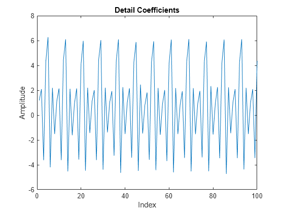
Use the lazy wavelet to obtain the even and odd polyphase components of the signal. Plot the detail (wavelet) coefficients in D, and observe that this transform has not decorrelated the signal. The wavelet coefficients look very much like the signal.
LS = liftingScheme;
[A,D] = lwt(x,'LiftingScheme',LS,'Level',1);
plot(D{1})
xlim([0 100])
title('Detail Coefficients')
xlabel('Index')
ylabel('Amplitude')

Add a prediction lifting step that subtracts the even-indexed coefficient from the odd-coefficient one sample later, .
ElemLiftStep = liftingStep('Type','predict','Coefficients',-1,'MaxOrder',0);
LSnew = addlift(LS,ElemLiftStep);
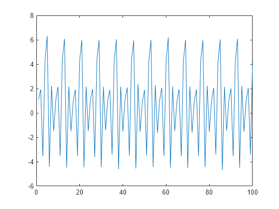
Because the signal is piecewise constant over consecutive samples with additive noise, the new prediction step should result in wavelet coefficients small in absolute value. In this case, the wavelet transform does decorrelate the data. Verify this by finding the approximation and detail coefficients with the new prediction step.
[A,D] = lwt(x,'liftingScheme',LSnew,'Level',1);
If you plot the detail (wavelet) coefficients, you see that the wavelet coefficients no longer resemble the original signal.
plot(D{1})
xlim([0 100])
title('Detail Coefficients')
xlabel('Index')
ylabel('Amplitude')
The approximation coefficients, A, of the previous transform constitute the even polyphase component of the signal. Therefore, the coefficients are affected by aliasing. Use an update lifting step to update the approximation coefficients and reduce aliasing. The update step replaces the approximation coefficients by , which is equal to the average of and . The averaging is a lowpass filtering, which helps to reduce aliasing.
ElemLiftStep = liftingStep('Type','update','Coefficients',1/2,'MaxOrder',0);
LSnew = addlift(LSnew,ElemLiftStep);
Use the new lifting scheme to obtain the wavelet transform of the input signal. The approximation coefficients resemble a smooth version of the original signal.
[A,D] = lwt(x,'liftingScheme',LSnew,'Level',1);
plot(A)
xlim([0 100])

Create a new lifting scheme with the same lifting steps as LSnew. Apply scaling factors to ensure perfect reconstruction. Obtain the approximation and wavelet coefficients using the lifting scheme and reconstruct the signal using ilwt. Verify perfect reconstruction.
scaleFactors = [sqrt(2) sqrt(2)/2];
ElemLiftStep1 = liftingStep('Type','predict','Coefficients',-1,'MaxOrder',0);
ElemLiftStep2 = liftingStep('Type','update','Coefficients',1/2,'MaxOrder',0);
LSscale = liftingScheme('LiftingSteps',[ElemLiftStep1;ElemLiftStep2], ...
    'NormalizationFactors',scaleFactors);
[A,D] = lwt(x,'liftingScheme',LSscale,'Level',1);
xrecon = ilwt(A,D,'liftingScheme',LSscale);
max(abs(x(:)-xrecon(:)))
ans =
1.7764e-15
The preceding example designed a wavelet, which effectively removed a zeroth order polynomial (constant). If the behavior of the signal is better represented by a higher-order polynomial, you can design a dual wavelet with the appropriate number of vanishing moments to decorrelate the signal.
Use the lifting scheme to design a wavelet with two vanishing moments. A dual wavelet with two vanishing moments decorrelates a signal with local behavior approximated by a first-order polynomial. Create a signal characterized by first-order polynomial behavior with additive noise.
y = [1 0 0 4 0 0 -1 0 0 2 0 0 7 0 0 -4 0 0 1 0 0 -3];
x1 = 1:(21/1024):22-(21/1024);
y1 = interp1(1:22,y,x1,'linear');
rng default
y1 = y1+0.25*randn(size(y1));
plot(x1,y1)
xlim([1 22])

In this case, the wavelet coefficients should remove a first-order polynomial. If the signal value at an odd index, , is well approximated by a first-order polynomial fitted to the surrounding sample values, then should provide a good fit for . In other words, should be the midpoint between and .
It follows that should decorrelate the signal.
Create a new lifting scheme with the prediction lifting step which models the preceding equation.
ElemLiftStep = liftingStep('Type','predict','Coefficients',[-1/2 -1/2],'MaxOrder',1);
LS = liftingScheme('LiftingSteps',ElemLiftStep,'NormalizationFactors',1);
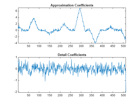
Use the lifting scheme to obtain the approximation and detail coefficients and plot the result.
[A,D] = lwt(y1,'LiftingScheme',LS,'Level',1);
subplot(2,1,1)
plot(A)
xlim([1 512])
title('Approximation Coefficients')
subplot(2,1,2)
plot(D{1})
xlim([1 512])
title('Detail Coefficients')

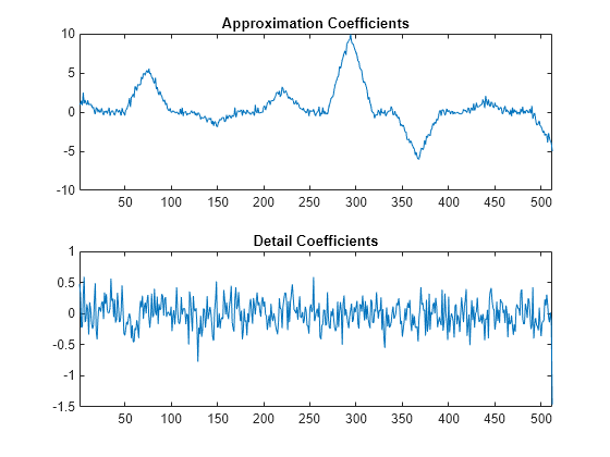
You see that the wavelet coefficients appear to only contain noise, while the approximation coefficients represent a denoised version of the original signal. Because the preceding transform uses only the even polyphase component for the approximation coefficients, you can reduce aliasing by adding an update step.
Create a new lifting scheme that consists of the previous prediction step and a new update step that reduces aliasing. Normalize the lifting scheme to produce a perfect reconstruction filter bank. Obtain the discrete wavelet transform with the new lifting scheme and plot the results.
scaleFactors = [sqrt(2) sqrt(2)/2];
ElemLiftStep1 = liftingStep('Type','predict','Coefficients',[-1/2 -1/2],'MaxOrder',1);
ElemLiftStep2 = liftingStep('Type','update','Coefficients',[1/4 1/4],'MaxOrder',0);
LSnew = liftingScheme('LiftingSteps',[ElemLiftStep1;ElemLiftStep2], ...
    'NormalizationFactors',scaleFactors);
[A,D] = lwt(y1,'liftingScheme',LSnew,'Level',1);
subplot(2,1,1)
plot(A)
xlim([1 512])
title('Approximation Coefficients')
subplot(2,1,2)
plot(D{1})
xlim([1 512])
title('Detail Coefficients')

Demonstrate that you have designed a perfect reconstruction filter bank.
y2 = ilwt(A,D,'liftingScheme',LSnew);
max(abs(y2(:)-y1(:)))
ans = 1.7764e-15