Harris Corner Detection
This example shows how to use edge detection as the first step in corner detection. The algorithm is suitable for FPGAs.
Corner detection is used in computer vision systems to find features in an image. It is often one of the first steps in applications like motion detection, tracking, image registration and object recognition.
A corner is intuitively defined as the intersection of two edges. This example uses the Harris & Stephens algorithm [ 1 ] in which the computation is simplified using an approximation of the eigenvalues of the Harris matrix. For another corner detection algorithm for FPGAs, see the FAST Corner Detection example.
This example model provides a hardware-compatible algorithm. You can implement this algorithm on a board using an AMD™ Zynq™ reference design. See Corner Detection and Image Overlay with Zynq-Based Hardware (SoC Blockset).
Introduction
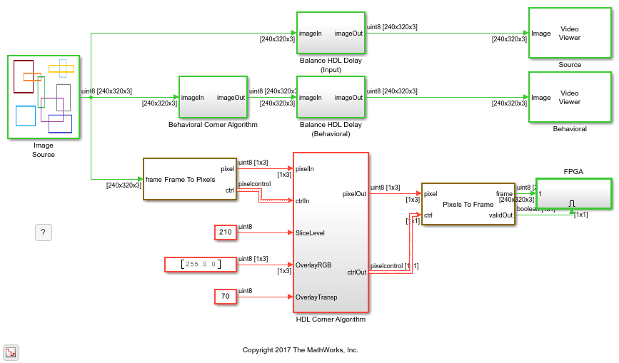
The CornerDetectionHDL.slx system is shown. The HDL Corner Algorithm subsystem contains a Corner Detector block with the Method parameter set to Harris.
First Step: Find the Gradients
The first step in the Harris algorithm is to find the edges in the image. The Corner Detector block uses two gradient image filters with coefficients ![$\left[ \begin{array}{ccc} {1}&{0}&{- 1} \end{array} \right]$](../../examples/visionhdl/win64/CornerDetectionHDLExample_eq06622402019137691954.png) and
and ![$\left[ \begin{array}{c} {1}\\{0}\\{- 1} \end{array} \right]$](../../examples/visionhdl/win64/CornerDetectionHDLExample_eq13614253029715706778.png) to produce gradients
to produce gradients  and
and  . Square and cross-multiply to form
  ,
,  and
and  .
.
Second Step: Circular Filtering
The second step of the algorithm is to perform Gaussian filtering to average , and over a circular window. The size of the circular window determines the scale of the detected corner. The block uses a 5x5 window. For three components, the block uses three filters with the same filter coefficients.
Final Step: Form the Harris Matrix
The final step of the algorithm is to estimate the eigenvalue of the Harris matrix. The Harris matrix is a symmetric matrix similar to a covariance matrix. The main diagonal is composed of the two averages of the gradients squared  and
and  . The off diagonal elements are the averages of the gradient cross-product
  . The Harris matrix is:
![$$A_{Harris} = \left[ {\begin{array}{*{20}{c}}{\langle G_x^2 \rangle}&{\langle G_{xy} \rangle}\\{\langle G_{xy} \rangle}&{\langle G_y^2 \rangle}\end{array}} \right]$$](../../examples/visionhdl/win64/CornerDetectionHDLExample_eq12372106257516886756.png)
Compute the Response from the Harris Matrix
The key simplification of the Harris algorithm is estimating the eigenvalues of the Harris matrix as the determinant minus the scaled trace squared.
 where
where  is a constant typically 0.04.
The corner metric response,  , expressed using the gradients is:

When the response is larger than a predefined threshold, a corner is detected:


Fixed-Point Settings
The overall function from input image to output corner metric response is a fourth-order polynomial. This leads to some challenges determining the fixed-point scaling for each step of the computation. Since we are targeting FPGAs with built-in multipliers, the best strategy is to allow bit growth until the multiplier size is reached and then start to quantize results on a selective basis to stay within the bounds of the provided multipliers.
The input pixel stream is 8-bit grayscale pixel data. Computing the gradients does not add much bit-growth since the filter kernel has only +1 and -1 coefficients. The result is a full-precision 9-bit signed fixed-point type.
Squaring and cross-multiplying the gradients produces signed 18-bit results, still in full precision. Many common FPGA multipliers have 18-bit or 20-bit input wordlengths, so you will have to quantize at the next step.
The next step is to apply a circular window to the three components using three Image Filters with Gaussian coefficients. The coefficients are quantized to 18-bit unsigned numbers to fit the FPGA multipliers. To find the best fraction precision for the coefficients, create a fixed-point number using the fi() function but only specifying the wordlength. In this case a fractional scaling of 21-bits is best since the largest value in the coefficient matrix is between 1/8 and 1/16.
coeffs = fi(fspecial('gaussian',[5,5],1.5),0,18)
coeffs =

    0.0144    0.0281    0.0351    0.0281    0.0144
    0.0281    0.0547    0.0683    0.0547    0.0281
    0.0351    0.0683    0.0853    0.0683    0.0351
    0.0281    0.0547    0.0683    0.0547    0.0281
    0.0144    0.0281    0.0351    0.0281    0.0144

          DataTypeMode: Fixed-point: binary point scaling
            Signedness: Unsigned
            WordLength: 18
        FractionLength: 21

Results of the Simulation
You can see that the resulting images from the simulation are very similar but not exactly the same. The small differences in simulation results are because the behavioral model uses C integer arithmetic rules and the quantization is different from the HDL-ready corner detection block.
Using Simulink, you can understand these differences and decide if the errors are allowable for your application. If they are not acceptable, you can increase the bit-widths of the operators, although this increases the area used in the FPGA.
HDL Code Generation
To check and generate the HDL code referenced in this example, you must have an HDL Coder™ license.
To generate the HDL code, use the following command.
makehdl('CornerDetectionHDL/HDL Corner Algorithm')
To generate the test bench, use the following command. Note that test bench generation takes a long time due to the large data size. You may want to reduce the simulation time before generating the test bench.
makehdltb('CornerDetectionHDL/HDL Corner Algorithm')
The part of this model that you can implement on an FPGA is the part between the Frame To Pixels and Pixels To Frame blocks. That is the subsystem called HDL Corner Algorithm, which includes all elements of the corner detection algorithm seen above. The rest of the model, including the Behavioral Corner Algorithm and the sources and sinks, form our Simulink test bench.
Going Further
The Harris & Stephens algorithm is based on approximating the eigenvalues of the Harris matrix as shown above. The Harris algorithm uses as a metric, avoiding any division or square-root operations. Another way to do corner detection is to compute the actual eigenvalues.
The analytical solution for the eigenvalues of a 2x2 matrix is well-known and can also be used in corner detection. When the eigenvalues are both positive and large with the same scale, a corner has been found.
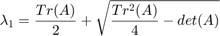

Substituting in our  values we get:
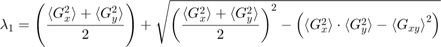

For FPGA implementation it is important to notice the repeated value of  . We can compute this value once and then square to combine with
  . This means that the eigenvalue algorithm requires only two multipliers but at the expense of more adders and subtractors and a square-root function, which requires several multipliers on its own.
You must then compare both eigenvalues to a constant value to make sure they are large. Since the eigenvalues scale up with image intensity, you also need to make sure they are both around the same size. You can do this by subtracting one from another and making sure that result is smaller than some predefined threshold value. Notice that in this subtraction, the first terms cancel out and you are left with:


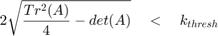

You can rearrange this so that it is very similar to Harris metric above:

Expanding the matrix gives:
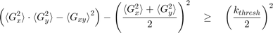
The similarity between the difference of the eigenvalues and the Harris metric shows how the Harris approximation works. If you rearrange the terms under the square-root and swap the signs so the result must be greater than or equal to a predefined threshold, you arrive at essentially the Harris metric with some scaling.
References
[1] C. Harris and M. Stephens (1988). "A combined corner and edge detector". Proceedings of the 4th Alvey Vision Conference. pp. 147-151.
See Also
Corner Detector | Pixel Stream Aligner