Main Content

vision.KalmanFilter

Correction of measurement, state, and state estimation error covariance

Description

The Kalman filter object is designed for tracking. You can use it to predict a physical object's future location, to reduce noise in the detected location, or to help associate multiple physical objects with their corresponding tracks. A Kalman filter object can be configured for each physical object for multiple object tracking. To use the Kalman filter, the object must be moving at constant velocity or constant acceleration.

Creation

The Kalman filter algorithm involves two steps, prediction and correction (also known as the update step). The first step uses previous states to predict the current state. The second step uses the current measurement, such as object location, to correct the state. The Kalman filter implements a discrete time, linear State-Space System.

Note

To make configuring a Kalman filter easier, you can use the configureKalmanFilter object to configure a Kalman filter. It sets up the filter for tracking a physical object in a Cartesian coordinate system, moving with constant velocity or constant acceleration. The statistics are the same along all dimensions. If you need to configure a Kalman filter with different assumptions, do not use the function, use this object directly.

In the state space system, the state transition model, A, and the measurement model, H, are set as follows:

VariableValue
A[1 1 0 0; 0 1 0 0; 0 0 1 1; 0 0 0 1]
H[1 0 0 0; 0 0 1 0]

Description

kalmanFilter = vision.KalmanFilter returns a kalman filter for a discrete time, constant velocity system.

example

kalmanFilter = vision.KalmanFilter(StateTransitionModel,MeasurementModel) additionally configures the control model, B.

kalmanFilter = vision.KalmanFilter(StateTransitionModel,MeasurementModel,ControlModel,Name,Value) configures the Kalman filter object properties, specified as one or more Name,Value pair arguments. Unspecified properties have default values.

Properties

expand all

Model describing state transition between time steps (A), specified as an M-by-M matrix. After the object is constructed, this property cannot be changed. This property relates to the A variable in the state-space model.

Model describing state to measurement transformation (H) , specified as an N-by-M matrix. After the object is constructed, this property cannot be changed. This property relates to the H variable in the state-space model.

Model describing control input to state transformation (B) , specified as an M-by-L matrix. After the object is constructed, this property cannot be changed. This property relates to the B variable in the state-space model.

State (x), specified as a scalar or an M-element vector. If you specify State as a scalar, it will be extended to an M-element vector. This property relates to the x variable in the state-space model.

State estimation error covariance (P), specified as a scalar or an M-by-M matrix. If you specify StateCovariance as a scalar it will be extended to an M-by-M diagonal matrix. This property relates to the P variable in the state-space system.

Process noise covariance (Q) , specified as a scalar or an M-by-M matrix. If you specify ProcessNoise as a scalar it will be extended to an M-by-M diagonal matrix. This property relates to the Q variable in the state-space model.

Measurement noise covariance (R) , specified as a scalar or an N-by-N matrix. If you specify MeasurementNoise as a scalar it will be extended to an N-by-N diagonal matrix. This property relates to the R variable in the state-space model.

Object Functions

Use the predict and correct functions based on detection results. Use the distance function to find the best matches.

  • When the tracked object is detected, use the predict and correct functions with the Kalman filter object and the detection measurement. Call the functions in the following order:

    [...] = predict(kalmanFilter);
    [...] = correct(kalmanFilter,measurement);

  • When the tracked object is not detected, call the predict function, but not the correct function. When the tracked object is missing or occluded, no measurement is available. Set the functions up with the following logic:

    [...] = predict(kalmanFilter);
    If measurement exists
    	[...] = correct(kalmanFilter,measurement);
    end

  • If the tracked object becomes available after missing for the past t-1 contiguous time steps, you can call the predict function t times. This syntax is particularly useful to process asynchronous video.. For example,

    for i = 1:k
      [...] = predict(kalmanFilter);
    end
    [...] = correct(kalmanFilter,measurement) 

correctCorrection of measurement, state, and state estimation error covariance
predictPrediction of measurement
distanceConfidence value of measurement

Examples

collapse all

Track the location of a physical object moving in one direction.

Generate synthetic data which mimics the 1-D location of a physical object moving at a constant speed.

detectedLocations = num2cell(2*randn(1,40) + (1:40));

Simulate missing detections by setting some elements to empty.

detectedLocations{1} = [];
  for idx = 16: 25 
      detectedLocations{idx} = []; 
  end

Create a figure to show the location of detections and the results of using the Kalman filter for tracking.

figure;
hold on;
ylabel('Location');
ylim([0,50]); 
xlabel('Time');
xlim([0,length(detectedLocations)]);

Figure contains an axes object. The axes object with xlabel Time, ylabel Location is empty.

Create a 1-D, constant speed Kalman filter when the physical object is first detected. Predict the location of the object based on previous states. If the object is detected at the current time step, use its location to correct the states.

kalman = []; 
for idx = 1: length(detectedLocations) 
   location = detectedLocations{idx}; 
   if isempty(kalman)
     if ~isempty(location) 
       
       stateModel = [1 1;0 1]; 
       measurementModel = [1 0]; 
       kalman = vision.KalmanFilter(stateModel,measurementModel,'ProcessNoise',1e-4,'MeasurementNoise',4);
      kalman.State = [location, 0]; 
     end 
   else
     trackedLocation = predict(kalman);
     if ~isempty(location) 
       plot(idx, location,'k+');
      d = distance(kalman,location); 
       title(sprintf('Distance:%f', d));
       trackedLocation = correct(kalman,location); 
     else 
       title('Missing detection'); 
     end 
     pause(0.2);
     plot(idx,trackedLocation,'ro'); 
   end 
 end 
legend('Detected locations','Predicted/corrected locations');

Figure contains an axes object. The axes object with title Distance:3.126145, xlabel Time, ylabel Location contains 66 objects of type line. One or more of the lines displays its values using only markers These objects represent Detected locations, Predicted/corrected locations.

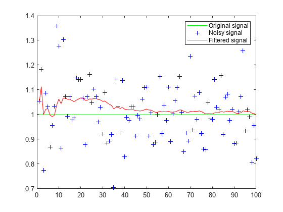
Use Kalman filter to remove noise from a random signal corrupted by a zero-mean Gaussian noise.

Synthesize a random signal that has value of 1 and is corrupted by a zero-mean Gaussian noise with standard deviation of 0.1.

x = 1;
len = 100;
z = x + 0.1 * randn(1,len);

Remove noise from the signal by using a Kalman filter. The state is expected to be constant, and the measurement is the same as state.

stateTransitionModel = 1;
measurementModel = 1;
obj = vision.KalmanFilter(stateTransitionModel,measurementModel,'StateCovariance',1,'ProcessNoise',1e-5,'MeasurementNoise',1e-2);

z_corr = zeros(1,len);
for idx = 1: len
 predict(obj);
 z_corr(idx) = correct(obj,z(idx));
end

Plot results.

figure, plot(x * ones(1,len),'g-'); 
hold on;
plot(1:len,z,'b+',1:len,z_corr,'r-');
legend('Original signal','Noisy signal','Filtered signal');

Figure contains an axes object. The axes object contains 3 objects of type line. One or more of the lines displays its values using only markers These objects represent Original signal, Noisy signal, Filtered signal.

Algorithms

expand all

References

[1] Welch, Greg, and Gary Bishop, An Introduction to the Kalman Filter, TR 95–041. University of North Carolina at Chapel Hill, Department of Computer Science.

[2] Blackman, S. Multiple-Target Tracking with Radar Applications. Artech House, Inc., pp. 93, 1986.

Extended Capabilities

Version History

Introduced in R2012b
Go to top of page