Animation and Solution of Double Pendulum Motion

Step 1: Define Displacement, Velocity, and Acceleration of Double Pendulum Masses

The following figure shows the model of a double pendulum. The double pendulum consists of two pendulum bobs and two rigid rods.

Describe the motion of the double pendulum by defining the state variables:

Describe the properties of the double pendulum by defining the variables:

For simplicity, ignore the masses of the two rigid rods. Specify all variables by using syms.

syms theta_1(t) theta_2(t) L_1 L_2 m_1 m_2 g

Define the displacements of the double pendulum in Cartesian coordinates.

x_1 = L_1*sin(theta_1);
y_1 = -L_1*cos(theta_1);
x_2 = x_1 + L_2*sin(theta_2);
y_2 = y_1 - L_2*cos(theta_2);

Find the velocities by differentiating the displacements with respect to time using the diff function.

vx_1 = diff(x_1);
vy_1 = diff(y_1);
vx_2 = diff(x_2);
vy_2 = diff(y_2);

Find the accelerations by differentiating the velocities with respect to time.

ax_1 = diff(vx_1);
ay_1 = diff(vy_1);
ax_2 = diff(vx_2);
ay_2 = diff(vy_2);

Step 2: Define Equations of Motion

Define the equations of motion based on Newton's laws.

First, specify the tension of the first rod as ${\mathit{T}}_1$, and the tension of the second rod ${\mathit{T}}_2$.

syms T_1 T_2

Next, construct free-body diagrams of the forces that act on both masses.

Evaluate the forces acting on ${\mathit{m}}_1$. Define the equations of motion of the first bob by balancing the horizontal and vertical force components. Specify these two equations as symbolic equations eqx_1 and eqy_1.

eqx_1 = m_1*ax_1(t) == -T_1*sin(theta_1(t)) + T_2*sin(theta_2(t))

eqx_1 = 
$$-m_1\hspace{0.17em}\left(L_1\hspace{0.17em}\sin \left({\theta }_1\left(t\right)\right)\hspace{0.17em}{\left(\frac{\partial }{\partial t}\mathrm{ }{\theta }_1\left(t\right)\right)}^2-L_1\hspace{0.17em}\cos \left({\theta }_1\left(t\right)\right)\hspace{0.17em}\frac{{\partial }^2}{\partial t^2}\mathrm{ }{\theta }_1\left(t\right)\right)=T_2\hspace{0.17em}\sin \left({\theta }_2\left(t\right)\right)-T_1\hspace{0.17em}\sin \left({\theta }_1\left(t\right)\right)$$

eqy_1 = m_1*ay_1(t) == T_1*cos(theta_1(t)) - T_2*cos(theta_2(t)) - m_1*g

eqy_1 = 
$$m_1\hspace{0.17em}\left(L_1\hspace{0.17em}\sin \left({\theta }_1\left(t\right)\right)\hspace{0.17em}\frac{{\partial }^2}{\partial t^2}\mathrm{ }{\theta }_1\left(t\right)+L_1\hspace{0.17em}\cos \left({\theta }_1\left(t\right)\right)\hspace{0.17em}{\left(\frac{\partial }{\partial t}\mathrm{ }{\theta }_1\left(t\right)\right)}^2\right)=T_1\hspace{0.17em}\cos \left({\theta }_1\left(t\right)\right)-g\hspace{0.17em}{m}_1-T_2\hspace{0.17em}\cos \left({\theta }_2\left(t\right)\right)$$

Evaluate the forces acting on ${\mathit{m}}_2$. Define the equations of motion of the second bob by balancing the horizontal and vertical force components. Specify these two equations as symbolic equations eqx_2 and eqy_2.

eqx_2 = m_2*ax_2(t) == -T_2*sin(theta_2(t))

eqx_2 = 
$$-m_2\hspace{0.17em}\left(L_1\hspace{0.17em}\sin \left({\theta }_1\left(t\right)\right)\hspace{0.17em}{\left(\frac{\partial }{\partial t}\mathrm{ }{\theta }_1\left(t\right)\right)}^2+L_2\hspace{0.17em}\sin \left({\theta }_2\left(t\right)\right)\hspace{0.17em}{\left(\frac{\partial }{\partial t}\mathrm{ }{\theta }_2\left(t\right)\right)}^2-L_1\hspace{0.17em}\cos \left({\theta }_1\left(t\right)\right)\hspace{0.17em}\frac{{\partial }^2}{\partial t^2}\mathrm{ }{\theta }_1\left(t\right)-L_2\hspace{0.17em}\cos \left({\theta }_2\left(t\right)\right)\hspace{0.17em}\frac{{\partial }^2}{\partial t^2}\mathrm{ }{\theta }_2\left(t\right)\right)=-T_2\hspace{0.17em}\sin \left({\theta }_2\left(t\right)\right)$$

eqy_2 = m_2*ay_2(t) == T_2*cos(theta_2(t)) - m_2*g

eqy_2 = 
$$m_2\hspace{0.17em}\left(L_1\hspace{0.17em}\cos \left({\theta }_1\left(t\right)\right)\hspace{0.17em}{\left(\frac{\partial }{\partial t}\mathrm{ }{\theta }_1\left(t\right)\right)}^2+L_2\hspace{0.17em}\cos \left({\theta }_2\left(t\right)\right)\hspace{0.17em}{\left(\frac{\partial }{\partial t}\mathrm{ }{\theta }_2\left(t\right)\right)}^2+L_1\hspace{0.17em}\sin \left({\theta }_1\left(t\right)\right)\hspace{0.17em}\frac{{\partial }^2}{\partial t^2}\mathrm{ }{\theta }_1\left(t\right)+L_2\hspace{0.17em}\sin \left({\theta }_2\left(t\right)\right)\hspace{0.17em}\frac{{\partial }^2}{\partial t^2}\mathrm{ }{\theta }_2\left(t\right)\right)=T_2\hspace{0.17em}\cos \left({\theta }_2\left(t\right)\right)-g\hspace{0.17em}{m}_2$$

Step 3: Evaluate Forces and Reduce System Equations

Four equations of motion describe the kinematics of the double pendulum. Evaluate the forces acting on the rods and reduce the set of four equations to two equations.

The equations of motion have four unknowns: ${\theta }_1$, ${\theta }_2$, ${\mathit{T}}_1$, and ${\mathit{T}}_2$. Evaluate the two unknowns ${\mathit{T}}_1$ and ${\mathit{T}}_2$ from eqx_1 and eqy_1. Use solve function to find ${\mathit{T}}_1$ and ${\mathit{T}}_2$.

Tension = solve([eqx_1 eqy_1],[T_1 T_2]);

Substitute the solutions for ${\mathit{T}}_1$ and ${\mathit{T}}_2$ into eqx_2 and eqy_2.

eqRed_1 = subs(eqx_2,[T_1 T_2],[Tension.T_1 Tension.T_2]);
eqRed_2 = subs(eqy_2,[T_1 T_2],[Tension.T_1 Tension.T_2]);

The two reduced equations fully describe the pendulum motion.

Step 4: Solve System Equations

Solve the system equations to describe the pendulum motion.

First, define the values for the masses in $\mathrm{kg}$, the rod lengths in $\mathrm{m}$, and the gravity in $\mathrm{m}/{\mathrm{s}}^2$ (SI units). Substitute these values into the two reduced equations.

L_1 = 1;
L_2 = 1.5;
m_1 = 2;
m_2 = 1;
g = 9.8;
eqn_1 = subs(eqRed_1)

eqn_1 = 
$$\begin{array}{l}\cos \left({\theta }_1\left(t\right)\right)\hspace{0.17em}{\sigma }_1-\frac{3\hspace{0.17em}\sin \left({\theta }_2\left(t\right)\right)\hspace{0.17em}{\left(\frac{\partial }{\partial t}\mathrm{ }{\theta }_2\left(t\right)\right)}^2}{2}-\sin \left({\theta }_1\left(t\right)\right)\hspace{0.17em}{\left(\frac{\partial }{\partial t}\mathrm{ }{\theta }_1\left(t\right)\right)}^2+\frac{3\hspace{0.17em}\cos \left({\theta }_2\left(t\right)\right)\hspace{0.17em}\frac{{\partial }^2}{\partial t^2}\mathrm{ }{\theta }_2\left(t\right)}{2}=-\frac{2\hspace{0.17em}\sin \left({\theta }_2\left(t\right)\right)\hspace{0.17em}\left({\cos \left({\theta }_1\left(t\right)\right)}^2\hspace{0.17em}{\sigma }_1+{\sin \left({\theta }_1\left(t\right)\right)}^2\hspace{0.17em}{\sigma }_1+\frac{49\hspace{0.17em}\sin \left({\theta }_1\left(t\right)\right)}{5}\right)}{\cos \left({\theta }_1\left(t\right)\right)\hspace{0.17em}\sin \left({\theta }_2\left(t\right)\right)-\cos \left({\theta }_2\left(t\right)\right)\hspace{0.17em}\sin \left({\theta }_1\left(t\right)\right)}\\ \\ \mathrm{where}\\ \\ \mathrm{ }{\sigma }_1=\frac{{\partial }^2}{\partial t^2}\mathrm{ }{\theta }_1\left(t\right)\end{array}$$

eqn_2 = subs(eqRed_2)

eqn_2 = 
$$\begin{array}{l}\cos \left({\theta }_1\left(t\right)\right)\hspace{0.17em}{\left(\frac{\partial }{\partial t}\mathrm{ }{\theta }_1\left(t\right)\right)}^2+\frac{3\hspace{0.17em}\cos \left({\theta }_2\left(t\right)\right)\hspace{0.17em}{\left(\frac{\partial }{\partial t}\mathrm{ }{\theta }_2\left(t\right)\right)}^2}{2}+\sin \left({\theta }_1\left(t\right)\right)\hspace{0.17em}{\sigma }_1+\frac{3\hspace{0.17em}\sin \left({\theta }_2\left(t\right)\right)\hspace{0.17em}\frac{{\partial }^2}{\partial t^2}\mathrm{ }{\theta }_2\left(t\right)}{2}=\frac{2\hspace{0.17em}\cos \left({\theta }_2\left(t\right)\right)\hspace{0.17em}\left({\cos \left({\theta }_1\left(t\right)\right)}^2\hspace{0.17em}{\sigma }_1+{\sin \left({\theta }_1\left(t\right)\right)}^2\hspace{0.17em}{\sigma }_1+\frac{49\hspace{0.17em}\sin \left({\theta }_1\left(t\right)\right)}{5}\right)}{\cos \left({\theta }_1\left(t\right)\right)\hspace{0.17em}\sin \left({\theta }_2\left(t\right)\right)-\cos \left({\theta }_2\left(t\right)\right)\hspace{0.17em}\sin \left({\theta }_1\left(t\right)\right)}-\frac{49}{5}\\ \\ \mathrm{where}\\ \\ \mathrm{ }{\sigma }_1=\frac{{\partial }^2}{\partial t^2}\mathrm{ }{\theta }_1\left(t\right)\end{array}$$

The two equations are nonlinear second-order differential equations. To solve these equations, convert them to first-order differential equations by using the odeToVectorField function.

[V,S] = odeToVectorField(eqn_1,eqn_2);

The elements of the vector V represent the first-order differential equations that are equal to the time derivative of the elements of S. The elements of S are the state variables ${\theta }_2$, $\mathit{d}{\theta }_2/\mathrm{dt}$, ${\theta }_1$, and $\mathit{d}{\theta }_1/\mathrm{dt}$. The state variables describe the angular displacements and velocities of the double pendulum.

S

S = 
$$\left(\begin{array}{c}{\theta }_2\\ {\mathrm{Dtheta}}_2\\ {\theta }_1\\ {\mathrm{Dtheta}}_1\end{array}\right)$$

Next, convert the first order-differential equations to a MATLAB function with the handle M.

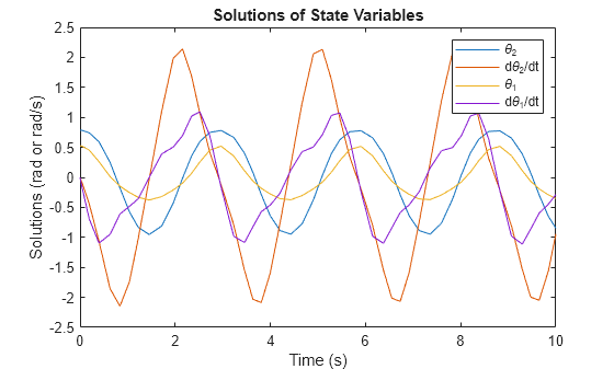
M = matlabFunction(V,'vars',{'t','Y'});

Define the initial conditions of the state variables as [pi/4 0 pi/6 0]. Use the ode45 function to solve for the state variables. The solutions are a function of time within the interval [0 10].

initCond = [pi/4 0 pi/6 0];
sols = ode45(M,[0 10],initCond);

Plot the solutions of the state variables.

plot(sols.x,sols.y)
legend('\theta_2','d\theta_2/dt','\theta_1','d\theta_1/dt')
title('Solutions of State Variables')
xlabel('Time (s)')
ylabel('Solutions (rad or rad/s)')

Step 5: Create Animation of Oscillating Double Pendulum

Create the animation of the oscillating double pendulum.

First, create four functions that use deval to evaluate the coordinates of both pendulums from the solutions sols.

x_1 = @(t) L_1*sin(deval(sols,t,3));
y_1 = @(t) -L_1*cos(deval(sols,t,3));
x_2 = @(t) L_1*sin(deval(sols,t,3))+L_2*sin(deval(sols,t,1));
y_2 = @(t) -L_1*cos(deval(sols,t,3))-L_2*cos(deval(sols,t,1));

Next, create a stop-motion animation object of the first pendulum bob by using the fanimator function. By default, fanimator creates an animation object with 10 generated frames per unit time within the range of t from 0 to 10. Plot the coordinates by using the plot function. Set the x-axis and y-axis to be equal length.

fanimator(@(t) plot(x_1(t),y_1(t),'ro','MarkerSize',m_1*10,'MarkerFaceColor','r'));
axis equal;

Next, add the animation objects of the first rigid rod, the second pendulum bob, and the second rigid rod.

hold on;
fanimator(@(t) plot([0 x_1(t)],[0 y_1(t)],'r-'));
fanimator(@(t) plot(x_2(t),y_2(t),'go','MarkerSize',m_2*10,'MarkerFaceColor','g'));
fanimator(@(t) plot([x_1(t) x_2(t)],[y_1(t) y_2(t)],'g-'));

Add a piece of text to count the elapsed time by using the text function. Use num2str to convert the time parameter to a string.

fanimator(@(t) text(-0.3,0.3,"Timer: "+num2str(t,2)));
hold off;

Use the command playAnimation to play the animation of the double pendulum.