Visualize High-Dimensional Data Using t-SNE

R2026b

This example shows how to visualize the humanactivity data, which consists of acceleration data collected from smartphones during various activities. tsne reduces the dimension of the data from 60 original dimensions to two or three. tsne creates a nonlinear transformation whose purpose is to enable grouping of points with similar characteristics. Ideally, the tsne result shows clean separation of the 60-dimensional data points into groups.

Load and Examine Data

Load the humanactivity data, which is available when you run this example.

load humanactivity

View a description of the data.

Description

Description = 29×1 string array
    "                        === Human Activity Data ===                        "
    "                                                                           "
    " The humanactivity data set contains 24,075 observations of five different "
    " physical human activities: Sitting, Standing, Walking, Running, and       "
    " Dancing. Each observation has 60 features extracted from acceleration     "
    " data measured by smartphone accelerometer sensors. The data set contains  "
    " the following variables:                                                  "
    "                                                                           "
    " * actid - Response vector containing the activity IDs in integers: 1, 2, "
    " 3, 4, and 5 representing Sitting, Standing, Walking, Running, and         "

The data set is organized by activity type. To better represent a random set of data, shuffle the rows.

n = numel(actid); % Number of data points
rng default % For reproducibility
idx = randsample(n,n); % Shuffle
X = feat(idx,:); % Shuffled data
actid = actid(idx); % Shuffled labels

Associate the activities with the labels in actid.

activities = ["Sitting";"Standing";"Walking";"Running";"Dancing"];
activity = activities(actid);

Reduce Dimension of Data to Two

Obtain two-dimensional analogues of the data clusters using t-SNE. To save time on this relatively large data set, use the Barnes-Hut variant of the t-SNE algorithm.

rng default % For reproducibility
Y = tsne(X,Algorithm="barneshut");

Display the result, colored with the correct labels.

figure
numGroups = length(unique(actid));
clr = hsv(numGroups);
gscatter(Y(:,1),Y(:,2),activity,clr)

t-SNE creates clusters of points based solely on their relative similarities. The clusters are not very well separated in this view.

Increase Perplexity

To obtain better separation between data clusters, try setting the Perplexity parameter to 300.

rng default % for reproducibility
Y = tsne(X,Algorithm="barneshut",Perplexity=300);
figure
gscatter(Y(:,1),Y(:,2),activity,clr)

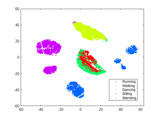
With the current settings, most of the clusters look better separated and structured. The sitting cluster comes in a few pieces, but these pieces are well-defined. The standing cluster is in two nearly circular pieces with very little data (colors) mixed in from other clusters. The walking cluster is one piece with a small admixture of colors from other activities. The dancing and running data are not separated from each other, but are mainly separated from the other data. This lack of separation means running and dancing are not easily distinguishable; perhaps this result is not surprising.

Reduce Dimension of Data to Three

t-SNE can also reduce the data to three dimensions. Set the tsne 'NumDimensions' argument to 3.

rng default % for fair comparison
Y3 = tsne(X,Algorithm="barneshut",Perplexity=300,NumDimensions=3);
figure
scatter3(Y3(:,1),Y3(:,2),Y3(:,3),15,clr(actid,:),'filled');
view(61,51)

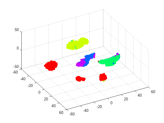
The clusters seem pretty well separated, with the exception of running and dancing. By rotating the 3-D plot, you can see that running and dancing are more easily distinguished in 3-D than in 2-D.