synthesizeTabularData
Syntax
Description
syntheticX = synthesizeTabularData(X,n)n observations of synthetic data using the existing data
X. The function returns the synthetic data
syntheticX. By default, synthesizeTabularData
uses a binning technique for generating synthetic data.
syntheticX = synthesizeTabularData(X,Yname,n)n observations of synthetic data using the existing data in
the table X and the class labels variable Yname in
X. (since R2026a)
[
generates syntheticX,syntheticY] = synthesizeTabularData(X,Y,n)n observations of synthetic data using the existing data
X and the class labels Y. The function returns
the synthetic data syntheticX and the synthetic class labels
syntheticY. (since R2026a)
___ = synthesizeTabularData(___,
specifies options using one or more name-value arguments in addition to any of the input
argument combinations in the previous syntaxes. For example, you can specify the synthetic
data generation method, the variables to use to generate synthetic data, and the options for
computing in parallel.Name=Value)
Examples
Generate synthetic data using an existing data set in a table. Visually compare the distributions of the existing and synthetic data sets.
Load the sample file fisheriris.csv, which contains iris data including sepal length, sepal width, petal width, and species type. Read the file into a table, and then convert the Species variable into a categorical variable. Display the first eight observations in the table.
fisheriris = readtable("fisheriris.csv");
fisheriris.Species = categorical(fisheriris.Species);
head(fisheriris)
SepalLength SepalWidth PetalLength PetalWidth Species
___________ __________ ___________ __________ _______
5.1 3.5 1.4 0.2 setosa
4.9 3 1.4 0.2 setosa
4.7 3.2 1.3 0.2 setosa
4.6 3.1 1.5 0.2 setosa
5 3.6 1.4 0.2 setosa
5.4 3.9 1.7 0.4 setosa
4.6 3.4 1.4 0.3 setosa
5 3.4 1.5 0.2 setosa
Create 1000 new observations from the data in fisheriris by using the synthesizeTabularData function. By default, the function uses a binning technique to learn the distribution of the variables in fisheriris before synthesizing data.
rng("default")
syntheticData = synthesizeTabularData(fisheriris,1000);
For each numeric variable, use box plots to visually compare the distribution of the values in fisheriris to the distribution of the values in syntheticData.
numericVariables = ["SepalLength","SepalWidth", ...
    "PetalLength","PetalWidth"];

boxchart(fisheriris{:,numericVariables})
hold on
boxchart(syntheticData{:,numericVariables})
hold off
legend(["Real data","Synthetic data"])
xticklabels(numericVariables)
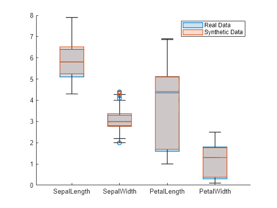
Blue box plots show the distributions of real data, and red box plots show the distributions of synthetic data. For each of the four numeric variables, the real and synthetic data values have similar distributions.
Use histograms to compare the distribution of flower species in fisheriris and syntheticData.
histogram(fisheriris.Species, ...
    Normalization="probability")
hold on
histogram(syntheticData.Species, ...
    Normalization="probability")
hold off
legend(["Real data","Synthetic data"])
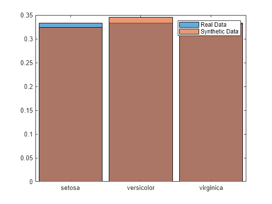
Overall, the distribution of flower species is similar across the two data sets. For example, 32% of the flowers in the synthetic data set are setosa irises, compared to 33% in the real data set.
Synthesize new data from existing training data by using a binning technique. Train a model using the existing training data, and then train the same type of model using the synthetic data. Compare the performance of the two models using test data.
Load the carbig data set, which contains measurements of cars made in the 1970s and early 1980s. Create a table containing the predictor variables Acceleration, Displacement, and so on, as well as the response variable MPG.
load carbig
tbl = table(Acceleration,Cylinders,Displacement,Horsepower, ...
    Model_Year,Origin,MPG,Weight);
Remove rows of tbl where the table has missing values.
tbl = rmmissing(tbl);
Partition the data into training and test sets. Use approximately 60% of the observations for model training and synthesizing new data, and 40% of the observations for model testing. Use cvpartition to partition the data.
rng("default")
cv = cvpartition(size(tbl,1),"Holdout",0.4);
trainTbl = tbl(training(cv),:);
testTbl = tbl(test(cv),:);
Synthesize new data from the trainTbl data set by using a binning technique. Specify to generate 1000 observations using 20 equal-width bins for each variable. Specify the Cylinders and Model_Year variables as discrete numeric variables.
syntheticTbl = synthesizeTabularData(trainTbl,1000, ...
    BinMethod="equal-width",NumBins=20, ...
    DiscreteNumericVariables=["Cylinders","Model_Year"]);
To visualize the difference between the existing data and synthetic data, you can use the detectdrift function. The function uses permutation testing to detect drift between trainTbl and syntheticTbl.
dd = detectdrift(trainTbl,syntheticTbl);
dd is a DriftDiagnostics object with plotEmpiricalCDF and plotHistogram object functions for visualization.
For continuous variables, use the plotEmpiricalCDF function to see the difference between the empirical cumulative distribution function (ecdf) of the values in trainTbl and the ecdf of the values in syntheticTbl.
continuousVariable ="Acceleration"; plotEmpiricalCDF(dd,Variable=continuousVariable) legend(["Real data","Synthetic data"])

For the Acceleration predictor, the ecdf plot for the existing values (in blue) matches the ecdf plot for the synthetic values (in red) fairly well.
For discrete variables, use the plotHistogram function to see the difference between the histogram of the values in trainTbl and the histogram of the values in syntheticTbl.
discreteVariable ="Cylinders"; plotHistogram(dd,Variable=discreteVariable) legend(["Real data","Synthetic data"])

For the Cylinders predictor, the histogram for the existing values (in blue) matches the histogram for the synthetic values (in red) fairly well.
Train a bagged ensemble of trees using the original training data trainTbl. Specify MPG as the response variable. Then, train the same kind of regression model using the synthetic data syntheticTbl.
originalMdl = fitrensemble(trainTbl,"MPG",Method="Bag");
newMdl = fitrensemble(syntheticTbl,"MPG",Method="Bag");
Evaluate the performance of the two models on the test set by computing the test mean squared error (MSE). Smaller MSE values indicate better performance.
originalMSE = loss(originalMdl,testTbl)
originalMSE =
7.0784
newMSE = loss(newMdl,testTbl)
newMSE =
6.1031
The model trained on the synthetic data performs slightly better on the test data.
Since R2026a
Synthesize new data from existing training data by using SMOTE (synthetic minority oversampling technique). Train a model using the existing training data, and then train the same type of model using both the existing training data and the synthetic data. Compare the performance of the two models using test data.
Load the carbig data set, which contains measurements of cars made in the 1970s and early 1980s. Categorize the cars based on whether they were made in Europe.
load carbig
Origin = categorical(cellstr(Origin));
Origin = mergecats(Origin,["France","Germany", ...
    "Sweden","Italy","England"],"Europe");
Origin = mergecats(Origin,["USA","Japan"],"NotEurope");
tabulate(Origin)
      Value    Count   Percent
     Europe       73     17.98%
  NotEurope      333     82.02%
The data is imbalanced, with only about 18% of cars originating in Europe.
Create a table containing the variables Acceleration, Displacement, and so on, as well as the response variable Origin. Remove rows of cars where the table has missing values.
cars = table(Acceleration,Displacement,Horsepower, ...
    MPG,Weight,Origin);
cars = rmmissing(cars);
Partition the data into training and test sets. Use approximately 50% of the observations for model training and synthesizing new data, and 50% of the observations for model testing. Use stratified partitioning so that approximately the same ratio of European to non-European cars exists in both the training and test sets.
rng("default")
cv = cvpartition(cars.Origin,Holdout=0.5);
trainCars = cars(training(cv),:);
testCars = cars(test(cv),:);
Synthesize new data from the trainCars data set by using SMOTE. Specify Origin as the class labels variable. Specify the ClassNames name-value argument to generate 40 synthetic observations belonging to the class of European cars only.
syntheticCars = synthesizeTabularData(trainCars, ...
    "Origin",40,Method="smote",ClassNames="Europe");
tabulate(syntheticCars.Origin)
      Value    Count   Percent
     Europe       40    100.00%
  NotEurope        0      0.00%
To visualize the difference between the existing European car data and the synthetic European car data, you can use the detectdrift function. Filter the trainCars data to include European car data only. The detectdrift function uses permutation testing to detect drift between europeanCars and syntheticCars.
europeanCars = trainCars(trainCars.Origin=="Europe",:);

dd = detectdrift(europeanCars,syntheticCars);
dd is a DriftDiagnostics object with a plotEmpiricalCDF object function for visualization.
For continuous variables, use the plotEmpiricalCDF function to see the difference between the empirical cumulative distribution function (ecdf) of the values in europeanCars and the ecdf of the values in syntheticCars.
continuousVariable ="Horsepower"; plotEmpiricalCDF(dd,Variable=continuousVariable) legend(["Real data","Synthetic data"])
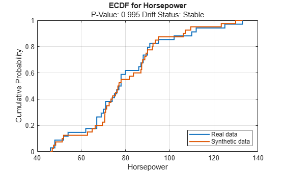
For the Horsepower predictor, the ecdf plot for the existing values (in blue) matches the ecdf plot for the synthetic values (in red) fairly well.
Train an SVM classifier using the original training data trainCars. Specify Origin as the response variable, and standardize the predictors before training. Then, train the same kind of classifier using both the original data and the synthetic data (syntheticCars).
originalMdl = fitcsvm(trainCars,"Origin",Standardize=true);
newMdl = fitcsvm([trainCars;syntheticCars],"Origin",Standardize=true);
Evaluate the performance of the two models on the test set using confusion matrices.
originalPredictions = predict(originalMdl,testCars);
newPredictions = predict(newMdl,testCars);

tiledlayout(1,2)
nexttile
confusionchart(testCars.Origin,originalPredictions)
title("Original Model")
nexttile
confusionchart(testCars.Origin,newPredictions)
title("New Model")
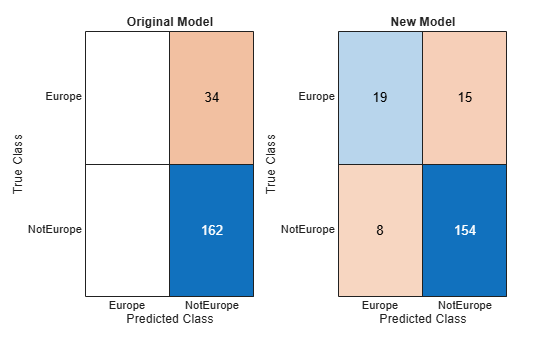
The model trained on the original data classifies all test observations as non-European cars. The model trained on the original and synthetic data has greater accuracy than the other model and correctly classifies the majority of European cars in the test set.
Evaluate data synthesized from an existing data set. Compare the existing and synthetic data sets to determine distribution similarity.
Load the carsmall data set. The file contains measurements of cars from 1970, 1976, and 1982. Create a table containing the data and display the first eight observations.
load carsmall
carData = table(Acceleration,Cylinders,Displacement,Horsepower, ...
    Mfg,Model,Model_Year,MPG,Origin,Weight);
head(carData)
    Acceleration    Cylinders    Displacement    Horsepower         Mfg                       Model                  Model_Year    MPG    Origin     Weight
    ____________    _________    ____________    __________    _____________    _________________________________    __________    ___    _______    ______

          12            8            307            130        chevrolet        chevrolet chevelle malibu                70        18     USA         3504
        11.5            8            350            165        buick            buick skylark 320                        70        15     USA         3693
          11            8            318            150        plymouth         plymouth satellite                       70        18     USA         3436
          12            8            304            150        amc              amc rebel sst                            70        16     USA         3433
        10.5            8            302            140        ford             ford torino                              70        17     USA         3449
          10            8            429            198        ford             ford galaxie 500                         70        15     USA         4341
           9            8            454            220        chevrolet        chevrolet impala                         70        14     USA         4354
         8.5            8            440            215        plymouth         plymouth fury iii                        70        14     USA         4312
Generate 100 new observations using the synthesizeTabularData function. Specify the Cylinders and Model_Year variables as discrete numeric variables. Display the first eight observations.
rng("default")
syntheticData = synthesizeTabularData(carData,100, ...
    DiscreteNumericVariables=["Cylinders","Model_Year"]);
head(syntheticData)
    Acceleration    Cylinders    Displacement    Horsepower         Mfg                       Model                  Model_Year     MPG      Origin     Weight
    ____________    _________    ____________    __________    _____________    _________________________________    __________    ______    _______    ______

       11.215           8           309.73         137.28      dodge            dodge coronet brougham                   76          17.3    USA          4038
       10.198           8           416.68         215.51      plymouth         plymouth fury iii                        70        9.5497    USA        4507.2
       17.161           6           258.38         77.099      amc              amc pacer d/l                            76        18.325    USA        3199.8
       9.4623           8           426.19          197.3      plymouth         plymouth fury iii                        70        11.747    USA        4372.1
       13.992           4           106.63         91.396      datsun           datsun pl510                             70         30.56    Japan      1950.7
       17.965           6           266.24         78.719      oldsmobile       oldsmobile cutlass ciera (diesel)        82        36.416    USA        2832.4
       17.028           4           139.02         100.24      chevrolet        chevrolet cavalier 2-door                82        36.058    USA        2744.5
       15.343           4           118.93         100.22      toyota           toyota celica gt                         82        26.696    Japan      2600.5
Visualize the synthetic and existing data sets. Create a DriftDiagnostics object using the detectdrift function. The object has the plotEmpiricalCDF and plotHistogram object functions you can use to visualize continuous and discrete variables.
dd = detectdrift(carData,syntheticData);
Use plotEmpiricalCDF to visualize the empirical cumulative distribution function (ECDF) of the values in carData and syntheticData.
continuousVariable ="Acceleration"; plotEmpiricalCDF(dd,Variable=continuousVariable) legend(["Real data","Synthetic data"])
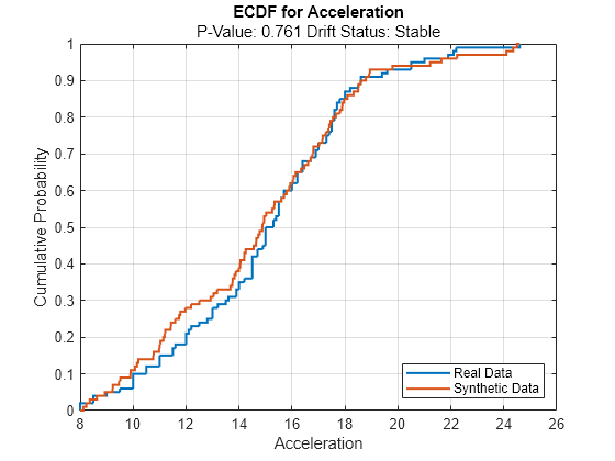
For the variable Acceleration, the ECDF of the existing data (in blue) and the ECDF of the synthetic data (in red) appear to be similar.
Use plotHistogram to visualize the distribution of values for discrete variables in carData and syntheticData.
discreteVariable ="Cylinders"; plotHistogram(dd,Variable=discreteVariable) legend(["Real data","Synthetic data"])
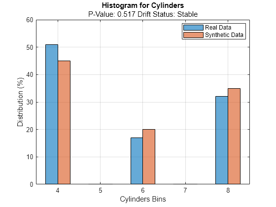
For the variable Cylinders, the distribution of data between the bins for the existing data (in blue) and the synthetic data (in red) appear similar.
Compare the synthetic and existing data sets using the mmdtest function. The function performs a two-sample hypothesis test for the null hypothesis that the samples come from the same distribution.
[mmd,p,h] = mmdtest(carData,syntheticData)
mmd =
0.0078
p =
0.8860
h =
0
The returned value of h = 0 indicates that mmdtest fails to reject the null hypothesis that the samples come from different distributions at the 5% significance level. As with other hypothesis tests, this result does not guarantee that the null hypothesis is true. That is, the samples do not necessarily come from the same distribution, but the low MMD value and high p-value indicate that the distributions of the real and synthetic data sets are similar.
Input Arguments
Name-Value Arguments
Output Arguments
Tips
Use SMOTE-based data generation when you have an imbalanced data set with mostly numeric predictors. If your data set contains only categorical predictors, consider using a different technique. For an example that shows different methods for handling imbalanced data, see Handle Class Imbalance in Binary Classification.
Algorithms
Alternative Functionality
Instead of calling the synthesizeTabularData function to generate
synthetic data directly, you can first create a binningTabularSynthesizer or smoteTabularSynthesizer object using an existing data set, and then call the
synthesizeTabularData object function to synthesize data using the object. By
creating an object, you can easily generate synthetic data multiple times without having to
relearn characteristics of the existing data set.
References
[1] Chawla, Nitesh V., Kevin W. Bowyer, Lawrence O. Hall, and W. Philip Kegelmeyer. "SMOTE: Synthetic Minority Over-sampling Technique." Journal of Artificial Intelligence Research 16 (2002): 321-357.