polyconf

Polynomial confidence intervals

Syntax

Y = polyconf(p,X)
[Y,DELTA] = polyconf(p,X,S)
[Y,DELTA] = polyconf(p,X,S,param1,val1,param2,val2,...)


Description

Y = polyconf(p,X) evaluates the polynomial p at the values in X. p is a vector of coefficients in descending powers.

[Y,DELTA] = polyconf(p,X,S) takes outputs p and S from polyfit and generates 95% prediction intervals Y ± DELTA for new observations at the values in X.

[Y,DELTA] = polyconf(p,X,S,param1,val1,param2,val2,...) specifies optional parameter name/value pairs chosen from the following list.

Parameter	Value
'alpha'	A value between 0 and 1 specifying a confidence level of 100*(1-alpha)%. The default is 0.05.
'mu'	A two-element vector containing centering and scaling parameters. With this option, polyconf uses (X-mu(1))/mu(2) in place of X.
'predopt'	Either 'observation' (the default) to compute prediction intervals for new observations at the values in X, or 'curve' to compute confidence intervals for the fit evaluated at the values in X. See below.
'simopt'	Either 'off' (the default) for nonsimultaneous bounds, or 'on' for simultaneous bounds. See below.

The 'predopt' and 'simopt' parameters can be understood in terms of the following functions:

• p(x) — the unknown mean function estimated by the fit

• l(x) — the lower confidence bound

• u(x) — the upper confidence bound

Suppose you make a new observation y_n+1 at x_n+1, so that

y_n+1(x_n+1) = p(x_n+1) + ε_n+1

By default, the interval [l_n+1(x_n+1), u_n+1(x_n+1)] is a 95% confidence bound on y_n+1(x_n+1).

The following combinations of the 'predopt' and 'simopt' parameters allow you to specify other bounds.

'simopt'	'predopt'	Bounded Quantity
'off'	'observation'	yn+1(xn+1) (default)
'off'	'curve'	p(xn+1)
'on'	'observation'	yn+1(x), for all x
'on'	'curve'	p(x), for all x

In general, 'observation' intervals are wider than 'curve' intervals, because of the additional uncertainty of predicting a new response value (the curve plus random errors). Likewise, simultaneous intervals are wider than nonsimultaneous intervals, because of the additional uncertainty of bounding values for all predictors x.

Examples

Plot Polynomial Fit and Prediction Intervals

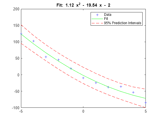
Fit a polynomial to a sample data set, and estimate the 95% prediction intervals and the roots of the fitted polynomial. Plot the data and the estimations, and display the fitted polynomial expression using the helper function polystr, whose code appears at the end of this example.

Generate sample data points (x,y) with a quadratic trend.

rng('default') % For reproducibility
x = -5:5;
y = x.^2 - 20*x - 3 + 5*randn(size(x));

Fit a second degree polynomial to the data by using polyfit.

degree = 2; % Degree of the fit
[p,S] = polyfit(x,y,degree);

Estimate the 95% prediction intervals by using polyconf.

alpha = 0.05; % Significance level
[yfit,delta] = polyconf(p,x,S,'alpha',alpha);

Plot the data, fitted polynomial, and prediction intervals. Display the fitted polynomial expression using the helper function polystr.

plot(x,y,'b+')
hold on
plot(x,yfit,'g-')
plot(x,yfit-delta,'r--',x,yfit+delta,'r--')
legend('Data','Fit','95% Prediction Intervals')
title(['Fit: ',texlabel(polystr(round(p,2)))])
hold off

Find the roots of the polynomial p.

r = roots(p)

r = 2×1

   17.5152
   -0.1017

Because the roots are real values, you can plot them as well. Estimate the fitted values and prediction intervals for the x interval that includes the roots. Then, plot the roots and the estimations.

if isreal(r)
    xmin = min([r(:);x(:)]);
    xrange = range([r(:);x(:)]);
    xExtended = linspace(xmin - 0.1*xrange, xmin + 1.1*xrange,1000);
    [yfitExtended,deltaExtended] = polyconf(p,xExtended,S,'alpha',alpha);

    plot(x,y,'b+')
    hold on
    plot(xExtended,yfitExtended,'g-')
    plot(r,zeros(size(r)),'ko')
    plot(xExtended,yfitExtended-deltaExtended,'r--')
    plot(xExtended,yfitExtended+deltaExtended,'r--')
    plot(xExtended,zeros(size(xExtended)),'k-')
    legend('Data','Fit','Roots of Fit','95% Prediction Intervals')
    title(['Fit: ',texlabel(polystr(round(p,2)))])
    axis tight
    hold off
end

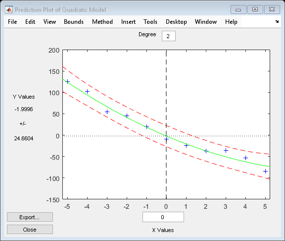
Alternatively, you can use polytool for interactive polynomial fitting.

polytool(x,y,degree,alpha)

Helper Function

The polystr.m file defines the polystr helper function.

type polystr.m % Display contents of polystr.m file

function s = polystr(p)
% POLYSTR Converts a vector of polynomial coefficients to a character string.
% S is the string representation of P.

if all(p == 0) % All coefficients are 0.
    s = '0';
else
    d = length(p) - 1; % Degree of polynomial.
    s = []; % Initialize s.
    for a = p
        if a ~= 0 % Coefficient is nonzero.
            if ~isempty(s) % String is not empty.
                if a > 0
                    s = [s ' + ']; % Add next term.
                else
                    s = [s ' - ']; % Subtract next term.
                    a = -a; % Value to subtract.
                end
            end
            if a ~= 1 || d == 0 % Add coefficient if it is ~=1 or polynomial is constant.
                s = [s num2str(a)];
                if d > 0 % For nonconstant polynomials, add *.
                    s = [s '*'];
                end
            end
            if d >= 2 % For terms of degree > 1, add power of x.
                s = [s 'x^' int2str(d)];
            elseif d == 1 % No power on x term.
                s = [s 'x'];
            end
        end
        d = d - 1; % Increment loop: Add term of next lowest degree.
    end
end
end

Version History

Introduced before R2006a