Nonlinear Regression Workflow

This example shows how to do a typical nonlinear regression workflow: import data, fit a nonlinear regression, test its quality, modify it to improve the quality, and make predictions based on the model.

Step 1. Prepare the data.

Load the reaction data.

load reaction

Examine the data in the workspace. reactants is a matrix with 13 rows and 3 columns. Each row corresponds to one observation, and each column corresponds to one variable. The variable names are in xn:

xn

xn = 3×10 char array
    'Hydrogen  '
    'n-Pentane '
    'Isopentane'

Similarly, rate is a vector of 13 responses, with the variable name in yn:

yn

yn = 
'Reaction Rate'

The hougen.m file contains a nonlinear model of reaction rate as a function of the three predictor variables. For a 5-D vector $$b$$ and 3-D vector $$x$$,

$$hougen(b,x)=\frac{b(1)x(2)-x(3)/b(5)}{1+b(2)x(1)+b(3)x(2)+b(4)x(3)}$$

As a start point for the solution, take b as a vector of ones.

beta0 = ones(5,1);

Step 2. Fit a nonlinear model to the data.

mdl = fitnlm(reactants,...
    rate,@hougen,beta0)

mdl = 
Nonlinear regression model:
    y ~ hougen(b,X)

Estimated Coefficients:
          Estimate       SE       tStat     pValue 
          ________    ________    ______    _______

    b1      1.2526     0.86702    1.4447    0.18654
    b2    0.062776    0.043562    1.4411    0.18753
    b3    0.040048    0.030885    1.2967    0.23089
    b4     0.11242    0.075158    1.4957    0.17309
    b5      1.1914     0.83671    1.4239     0.1923


Number of observations: 13, Error degrees of freedom: 8
Root Mean Squared Error: 0.193
R-Squared: 0.999,  Adjusted R-Squared 0.998
F-statistic vs. zero model: 3.91e+03, p-value = 2.54e-13

Step 3. Examine the quality of the model.

The root mean squared error is fairly low compared to the range of observed values.

[mdl.RMSE min(rate) max(rate)]

ans = 1×3

    0.1933    0.0200   14.3900

Examine a residuals plot.

plotResiduals(mdl)

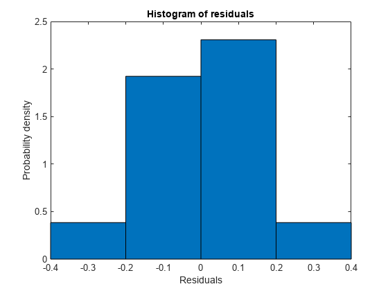
The model seems adequate for the data.

Examine a diagnostic plot to look for outliers.

plotDiagnostics(mdl,'cookd')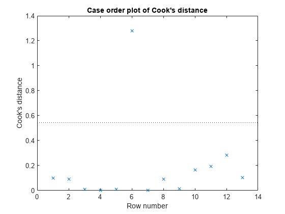

Observation 6 seems out of line.

Step 4. Remove the outlier.

Remove the outlier from the fit using the Exclude name-value pair.

mdl1 = fitnlm(reactants,...
    rate,@hougen,ones(5,1),'Exclude',6)

mdl1 = 
Nonlinear regression model:
    y ~ hougen(b,X)

Estimated Coefficients:
          Estimate       SE       tStat     pValue 
          ________    ________    ______    _______

    b1       0.619      0.4552    1.3598    0.21605
    b2    0.030377    0.023061    1.3172    0.22924
    b3    0.018927     0.01574    1.2024    0.26828
    b4    0.053411    0.041084       1.3    0.23476
    b5      2.4125      1.7903    1.3475     0.2198


Number of observations: 12, Error degrees of freedom: 7
Root Mean Squared Error: 0.198
R-Squared: 0.999,  Adjusted R-Squared 0.998
F-statistic vs. zero model: 2.67e+03, p-value = 2.54e-11

The model coefficients changed quite a bit from those in mdl.

Step 5. Examine slice plots of both models.

To see the effect of each predictor on the response, make a slice plot using plotSlice(mdl).

plotSlice(mdl)  

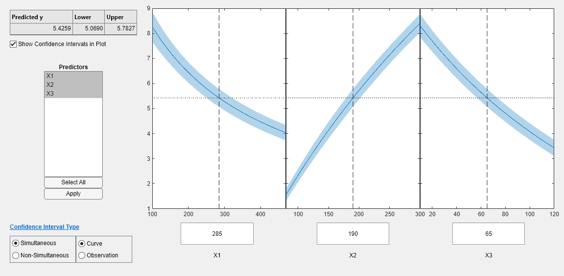
plotSlice(mdl1)  

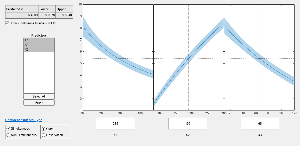
The plots look very similar, with slightly wider confidence bounds for mdl1. This difference is understandable, since there is one less data point in the fit, representing over 7% fewer observations.

Step 6. Predict for new data.

Create some new data and predict the response from both models.

Xnew =  [200,200,200;100,200,100;500,50,5];
[ypred yci] = predict(mdl,Xnew)

ypred = 3×1

    1.8762
    6.2793
    1.6718

yci = 3×2

    1.6283    2.1242
    5.9789    6.5797
    1.5589    1.7846

[ypred1 yci1] = predict(mdl1,Xnew)

ypred1 = 3×1

    1.8984
    6.2555
    1.6594

yci1 = 3×2

    1.6260    2.1708
    5.9323    6.5787
    1.5345    1.7843

Even though the model coefficients are dissimilar, the predictions are nearly identical.