Delete-1 Statistics
Delete-1 Change in Covariance (CovRatio)
Purpose
Delete-1 change in covariance (CovRatio) identifies the
observations that are influential in the regression fit. An influential
observation is one where its exclusion from the model might significantly alter
the regression function. Values of CovRatio larger than 1 +
3*p/n or smaller than 1 –
3*p/n indicate influential points,
where p is the number of regression coefficients, and
n is the number of observations.
Definition
The CovRatio statistic is the ratio of the determinant of
the coefficient covariance matrix with observation i deleted
to the determinant of the covariance matrix for the full model:
CovRatio is an n-by-1
vector in the Diagnostics table of the fitted
LinearModel object. Each element is the ratio of the
generalized variance of the estimated coefficients when the corresponding
element is deleted to the generalized variance of the coefficients using all the
data.
How To
After obtaining a fitted model, say, mdl, using
fitlm or stepwiselm, you can:
Display the
CovRatioby indexing into the property using dot notationmdl.Diagnostics.CovRatio
Plot the delete-1 change in covariance using
For details, see theplotDiagnostics(mdl,'CovRatio')
plotDiagnosticsmethod of theLinearModelclass.
Determine Influential Observations Using CovRatio
This example shows how to use the CovRatio statistics to determine the influential points in data. Load the sample data and define the response and predictor variables.
load hospital
y = hospital.BloodPressure(:,1);
X = double(hospital(:,2:5));
Fit a linear regression model.
mdl = fitlm(X,y);
Plot the CovRatio statistics.
plotDiagnostics(mdl,'CovRatio')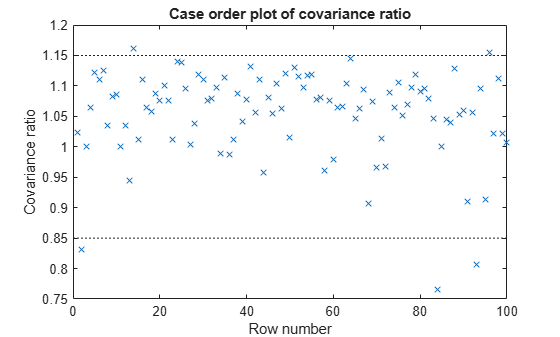
For this example, the threshold limits are 1 + 3*5/100 = 1.15 and 1 - 3*5/100 = 0.85. There are a few points beyond the limits, which might be influential points.
Find the observations that are beyond the limits.
find((mdl.Diagnostics.CovRatio)>1.15|(mdl.Diagnostics.CovRatio)<0.85)
ans = 5×1

     2
    14
    84
    93
    96
Delete-1 Scaled Difference in Coefficient Estimates (Dfbetas)
Purpose
The sign of a delete-1 scaled difference in coefficient estimate
(Dfbetas) for coefficient j and
observation i indicates whether that observation causes an
increase or decrease in the estimate of the regression coefficient. The absolute
value of a Dfbetas indicates the magnitude of the difference
relative to the estimated standard deviation of the regression coefficient. A
Dfbetas value larger than 3/sqrt(n) in
absolute value indicates that the observation has a large influence on the
corresponding coefficient.
Definition
Dfbetas for coefficient j and
observation i is the ratio of the difference in the estimate
of coefficient j using all observations and the one obtained
by removing observation i, and the standard error of the
coefficient estimate obtained by removing observation i. The
Dfbetas for coefficient j and
observation i is
where
bj is the
estimate for coefficient j,
bj(i)
is the estimate for coefficient j by removing observation
i,
MSE(i) is the
mean squared error of the regression fit by removing observation
i, and
hii is the
leverage value for observation i. Dfbetas
is an n-by-p matrix in the
Diagnostics table of the fitted
LinearModel object. Each cell of
Dfbetas corresponds to the Dfbetas
value for the corresponding coefficient obtained by removing the corresponding
observation.
How To
After obtaining a fitted model, say, mdl, using
fitlm or stepwiselm, you can obtain
the Dfbetas values as an
n-by-p matrix by indexing into the
property using dot
notation,
mdl.Diagnostics.Dfbetas
Determine Observations Influential on Coefficients Using Dfbetas
This example shows how to determine the observations that have large influence on coefficients using Dfbetas. Load the sample data and define the response and independent variables.
load hospital
y = hospital.BloodPressure(:,1);
X = double(hospital(:,2:5));
Fit a linear regression model.
mdl = fitlm(X,y);
Find the Dfbetas values that are high in absolute value.
[row,col] = find(abs(mdl.Diagnostics.Dfbetas)>3/sqrt(100));
disp([row col])
     2     1
    28     1
    84     1
    93     1
     2     2
    13     3
    84     3
     2     4
    84     4
Delete-1 Scaled Change in Fitted Values (Dffits)
Purpose
The delete-1 scaled change in fitted values (Dffits) show
the influence of each observation on the fitted response values.
Dffits values with an absolute value larger than
2*sqrt(p/n) might be influential.
Definition
Dffits for observation i is
where sri
is the studentized residual, and
hii is the
leverage value of the fitted LinearModel object.
Dffits is an n-by-1 column vector in
the Diagnostics table of the fitted
LinearModel object. Each element in
Dffits is the change in the fitted value caused by
deleting the corresponding observation and scaling by the standard error.
How To
After obtaining a fitted model, say, mdl, using
fitlm or stepwiselm, you can:
Display the
Dffitsvalues by indexing into the property using dot notationmdl.Diagnostics.Dffits
Plot the delete-1 scaled change in fitted values using
For details, see theplotDiagnostics(mdl,'Dffits')
plotDiagnosticsmethod of theLinearModelclass for details.
Determine Observations Influential on Fitted Response Using Dffits
This example shows how to determine the observations that are influential on the fitted response values using Dffits values. Load the sample data and define the response and independent variables.
load hospital
y = hospital.BloodPressure(:,1);
X = double(hospital(:,2:5));
Fit a linear regression model.
mdl = fitlm(X,y);
Plot the Dffits values.
plotDiagnostics(mdl,'Dffits')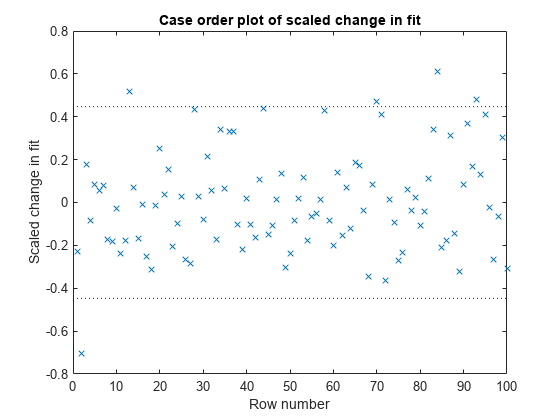
The influential threshold limit for the absolute value of Dffits in this example is 2*sqrt(5/100) = 0.45. Again, there are some observations with Dffits values beyond the recommended limits.
Find the Dffits values that are large in absolute value.
find(abs(mdl.Diagnostics.Dffits)>2*sqrt(4/100))
ans = 10×1

     2
    13
    28
    44
    58
    70
    71
    84
    93
    95
Delete-1 Variance (S2_i)
Purpose
The delete-1 variance (S2_i) shows how the mean squared
error changes when an observation is removed from the data set. You can compare
the S2_i values with the value of the mean squared
error.
Definition
S2_i is a set of residual variance estimates obtained by
deleting each observation in turn. The S2_i value for
observation i is
where
yj is the
jth observed response value. S2_i is
an n-by-1 vector in the Diagnostics table
of the fitted LinearModel object. Each element in
S2_i is the mean squared error of the regression obtained
by deleting that observation.
How To
After obtaining a fitted model, say, mdl, using
fitlm or stepwiselm, you can:
Display the
S2_ivector by indexing into the property using dot notationmdl.Diagnostics.S2_i
Plot the delete-1 variance values using
For details, see theplotDiagnostics(mdl,'S2_i')
plotDiagnosticsmethod of theLinearModelclass.
Compute and Examine Delete-1 Variance Values
This example shows how to compute and plot S2_i values to examine the change in the mean squared error when an observation is removed from the data. Load the sample data and define the response and independent variables.
load hospital
y = hospital.BloodPressure(:,1);
X = double(hospital(:,2:5));
Fit a linear regression model.
mdl = fitlm(X,y);
Display the MSE value for the model.
mdl.MSE
ans =
23.1140
Plot the S2_i values.
plotDiagnostics(mdl,'S2_i')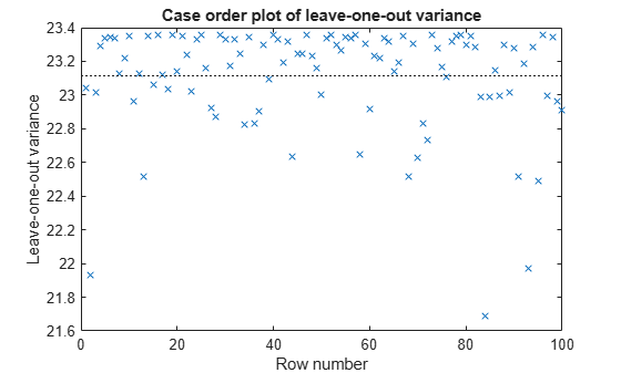
This plot makes it easy to compare the S2_i values to the MSE value of 23.114, indicated by the horizontal dashed lines. You can see how deleting one observation changes the error variance.
See Also
LinearModel | fitlm | stepwiselm | plotDiagnostics | plotResiduals