Parameter Estimation for Power Plant Excitation System Starting at Steady-State (GUI)
This example shows how to perform parameter estimation while starting the system in steady state using the example of an excitation system model for a power plant electric generator.
Need for Parameter Estimation in Power Systems
Parameter estimation is a powerful tool for power system operations where the accuracy of models is critical and may be required by regulation. There are several reasons why one might need to perform parameter estimation in power systems, including:
The system parameters may have been unknown from the start. For instance, if some or all of the parameters were not provided by the supplier.
Even if the system parameters were known in the past, these parameters may drift with time due to wear on components in the system.
Some settings may be changed for the system causing unknown effects on the system parameters. Parameter estimation can be used to account for these settings changes.
The system may need to be fit to some standardized model. For instance, in this example we are fitting the IEEE DC1A standard model for excitation systems to our system.
Excitation System Model Description
Generators create power by rotating a magnetic field and coiled wires relative to one another to induce an electric current. For generators that use electromagnets, an excitation system supplies current to the generator's field coils to create the magnetic field. By controlling the strength of the magnetic field inside the generator, the exciter system can control the generator's output voltage.
The Simulink® model spe_exciter models an excitation system in an offline step test. In this test, the generator is taken offline, then a step voltage input is applied to the exciter, and the output voltage is measured for system characterization purposes. This model includes the subsystem labeled "DC1A Excitation System" which follows the model structure for an excitation system outlined in the IEEE DC1A standard. The block contains several parameters, such as gains and time constants, that define the system's behavior and need to be fit to our system. The voltage inputs and outputs are in p.u. (per unit).
You can open the model with the following command:
open_system('spe_exciter');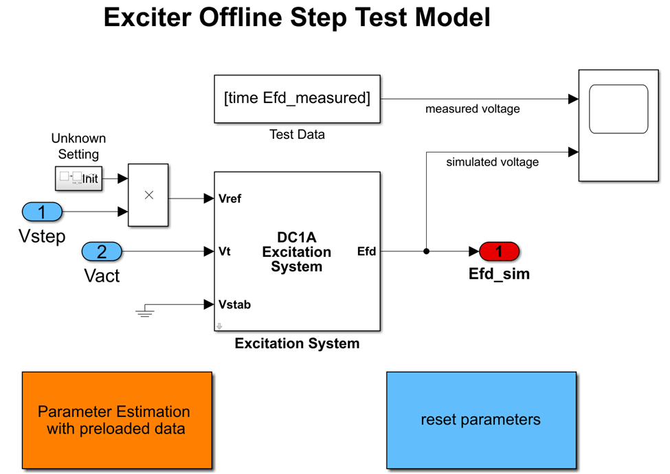
Open Parameter Estimator App
Double-click the orange block labeled Parameter Estimation with preloaded data in the lower left corner of the model. This will launch a Parameter Estimation session pre-loaded with data for this project, including the experimental data from the offline step test.
The Parameter Estimation session is loaded with the system parameters which were determined to need tuning due to any of the reasons noted previously. These parameters include the gains Ka, Ke, and Kf; and time constants Ta, Tb, Tc, Te, Tf, and Tr. These parameters are bound to use only positive values during estimation.
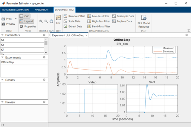
To plot the model's response against the experimental data, click the Plot Model Response button in the toolbar. Notice that the initial conditions for the states in our model are currently incorrect, which causes the initial dynamic in the simulated response and the offset between the simulated and measured response. In the next step we will update the options in the Parameter Estimator app to solve for the correct initial conditions in our model.
Compute Steady-State Operating Point During Parameter Estimation
In the experimental step test that produced the measured response, the excitation system was in steady state and outputting around 1.1 p.u. before the test measurements began. To match these conditions in our parameter estimation, we will specify that the model should start at a steady-state operating point during parameter estimation. Click More Options and select Operating Point Options.

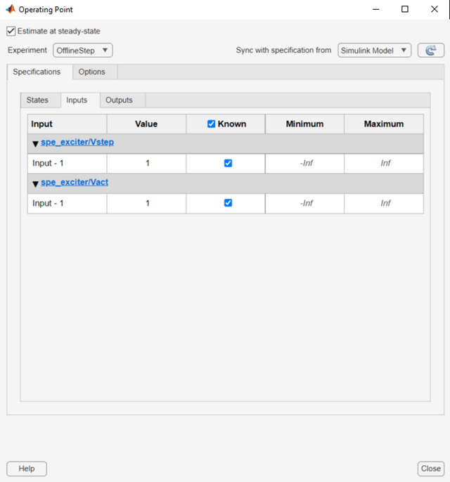
This shows a dialog box where you can specify how steady-state operating points should be computed during parameter estimation. Open the dialog box and select the check box Estimate at steady-state so that the Parameter Estimator will put the model into steady-state each time it varies parameters and runs the model. There are six states in this model, by default they will be set to unknown and marked as states to be set to steady-state. This matches our system, so we will keep these options unchanged.

The inputs to the model (terminal voltage and reference voltage) are known from the offline step test. Switching to the Inputs tab under Specifications, we can specify these conditions. We can see that the inputs are marked as known by default with a value of one. These come from the starting value in the measured data, and we will leave these values unchanged.
Switching to the Outputs tab under Specifications, we mark the output (field voltage) of our system as known by checking the “Known” checkbox, and set its “Value” to 1.1028, which is the first value of our measured field voltage test data.

With the options we have now set up, before running each model simulation, Parameter Estimation will solve for a set of initial conditions that will place all the specified states in steady-state at the specified input and output levels. To see the result of these changes, click Plot Model Response again and see that the simulated response is now in steady state at the expected initial output.

Set Up Parameter Estimation View
Before estimating parameters, we can use the toolbar to customize the view of Parameter Estimation to display the information we are interested in. Use the Add Plot button on the toolbar to add a Parameter Trajectory plot and an Estimation Cost plot. You can use the View tab to adjust the layout and make all plots visible.

Perform Parameter Estimation
Now we are ready to perform parameter estimation. In the Parameter Estimation tab, click Estimate. Due to the large number of parameters being estimated in this example, this process may take several minutes.
Once the estimation process has converged, the new model response is shown in the Experiment Plot. We see a better match between the model and the measured data, and the error in the ExpCost plot decreased significantly. These indicate that a good set of parameters was found. The EstimatedParams plot shows how each parameter changed at each iteration. To more clearly see how much each parameter changed relative to its initial value, right click the EstimatedParams plot and select Show scaled values.

Speed Up Estimation Using Parallel Pool Options
Because of the large number of parameters being estimated, the parameter estimation can take a long time. As the number of parameters increases, the number of times the model must run at each iteration also increases. This leads to an increase in the total computation time required for the parameter estimation to converge.
To speed up our parameter estimation we can set up our options to use a parallel pool. Then our parallel workers can run simulations simultaneously to speed up the parameter estimation process.
To do this you will need MATLAB Parallel Computing Toolbox. Before performing parameter estimation, go to More Options>Parallel Options in the Parameter Estimation toolbar. Then select Use parallel pool during estimation. Click OK, then click Estimate in the toolbar.
For a parallel pool with 8 workers, the estimation process for this example was 3.5 times faster to complete. For access to options related to parallel computing like number of workers and cluster setup, see Specify Your Parallel Settings (Parallel Computing Toolbox).