Estimate Model Parameters with Parameter Constraints (Code)

This example shows how to estimate model parameters while imposing constraints on the parameter values.

You estimate dynamic and static friction coefficients of a simple friction system.

Open the Model and Get Experimental Data

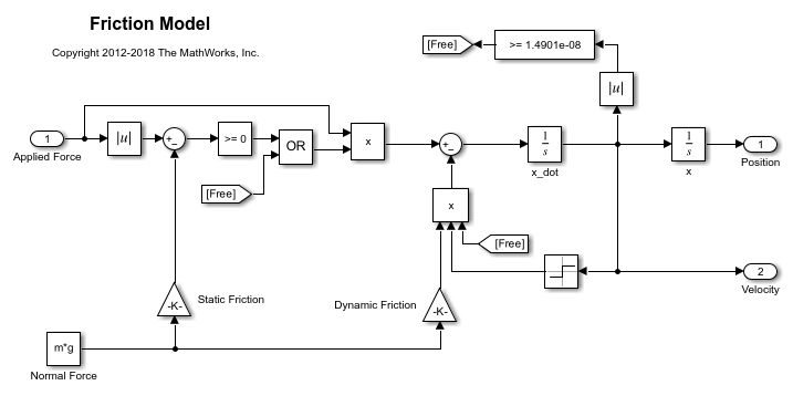
This example estimates parameters for a simple friction system, sdoFriction. The model input is the force applied to a mass and the model outputs are the mass position and velocity.

open_system('sdoFriction');

The model is based on a mass sliding on a surface. The mass is subject to a static friction that must be overcome before the mass moves and a dynamic friction once the mass moves. The static friction, u_static, is a fraction of the mass normal force; similarly the dynamic friction, u_dynamic, is a fraction of the mass normal force.

Load the experiment data. The mass was subjected to an applied force and its position recorded.

load sdoFriction_ExperimentData

The variables AppliedForce, Position, and Velocity are loaded into the workspace. The first column of each of these variables represents time and the second column represents the measured data. Because velocity is the first derivative of position, only use the position measurements for this example.

Plot the Experiment Data

subplot(211),
plot(AppliedForce(:,1),AppliedForce(:,2))
title('Measured Applied Force Input for Simple Friction System');
ylabel('Applied Force (N)')
subplot(212)
plot(Position(:,1),Position(:,2))
title('Measured Mass Position for Simple Friction System');
xlabel('Time (seconds)')
ylabel('Position (m)')

Define the Estimation Experiment

Create an experiment object to specify the experiment data.

Exp = sdo.Experiment('sdoFriction');

Specify the input data (applied force) as a timeseries object.

Exp.InputData = timeseries(AppliedForce(:,2),AppliedForce(:,1));

Create an object to specify the measured mass position output.

PositionSig = Simulink.SimulationData.Signal;
PositionSig.Name      = 'Position';
PositionSig.BlockPath = 'sdoFriction/x';
PositionSig.PortType  = 'outport';
PositionSig.PortIndex = 1;
PositionSig.Values    = timeseries(Position(:,2),Position(:,1));

Add the measured mass position data to the experiment as the expected output data.

Exp.OutputData = PositionSig;

Compare the Measured Output and the Initial Simulated Output

Create a simulation scenario using the experiment and obtain the simulated output.

Simulator    = createSimulator(Exp);
Simulator    = sim(Simulator);

Search for the position signal in the logged simulation data.

SimLog     = find(Simulator.LoggedData,get_param('sdoFriction','SignalLoggingName'));
Position   = find(SimLog,'Position');

Plot the measured and simulated data.

As expected, the model response does not match the experimental output data.

figure
plot(...
    Position.Values.Time,Position.Values.Data, ...
    Exp.OutputData.Values.Time, Exp.OutputData.Values.Data,'-.')
title('Simulated and Measured Responses Before Estimation')
ylabel('Position (m)')
xlabel('Time (seconds)')
legend('Simulated Position','Measured Position','Location','NorthWest')

Specify Parameters to Estimate

Estimate the u_static and u_dynamic friction coefficients using the experiment data. These coefficients are used as gains in the Static Friction and Dynamic Friction blocks, respectively. Physics indicates that friction coefficients should be constrained so that u_static $\geq$ u_dynamic; this parameter constraint is implemented in the estimation objective function.

Select the u_static and u_dynamic model parameters. Specify bounds for the estimated parameter values. Both coefficients are limited to the range [0 1].

p = sdo.getParameterFromModel('sdoFriction',{'u_static','u_dynamic'});

p(1).Minimum = 0;
p(1).Maximum = 1;

p(2).Minimum = 0;
p(2).Maximum = 1;

Define the Estimation Objective

Create an estimation objective function to evaluate how closely the simulation output, generated using the estimated parameter values, matches the measured data.

Use an anonymous function with one input argument that calls the sdoFriction_Objective function. We pass the anonymous function to sdo.optimize, which evaluates the function at each optimization iteration.

estFcn = @(v) sdoFriction_Objective(v,Simulator,Exp);

The sdoFriction_Objective function:

Has one input argument that specifies the estimated friction coefficients.

Has one input argument that specifies the experiment object containing the measured data.

Returns the sum-squared-error errors between simulated and experimental outputs, and returns the parameter constraint.

The sdoFriction_Objective function requires two inputs, but sdo.optimize requires a function with one input argument. To work around this, estFcn is an anonymous function with one input argument, v, but it calls sdoFriction_Objective using two input arguments, v and Exp.

For more information regarding anonymous functions, see Anonymous Functions.

The sdo.optimize command minimizes the return argument of the anonymous function estFcn, that is, the residual errors returned by sdoFriction_Objective. For more details on how to write an objective/constraint function to use with the sdo.optimize command, type help sdoExampleCostFunction at the MATLAB® command prompt.

To examine the estimation objective function in more detail, type edit sdoFriction_Objective at the MATLAB command prompt.

type sdoFriction_Objective

function vals = sdoFriction_Objective(p,Simulator,Exp) 
%SDOFRICTION_OBJECTIVE
%
%    The sdoFriction_Objective function is used to compare model
%    outputs against experimental data and measure how well constraints are
%    satisfied.
%
%    vals = sdoFriction_Objective(p,Exp) 
%
%    The |p| input argument is a vector of estimated model parameter values.
%
%    The |Simulator| input argument is a simulation object used 
%    simulate the model with the estimated parameter values.
%
%    The |Exp| input argument contains the estimation experiment data.
%
%    The |vals| return argument contains information about how well the
%    model simulation results match the experimental data and how well
%    constraints are satisfied. The |vals| argument is used by the
%    |sdo.optimize| function to estimate the model parameters.
%
%    See also sdo.optimize, sdoExampleCostFunction, sdoFriction_cmddemo
%
 
% Copyright 2012-2015 The MathWorks, Inc.

%%
% Define a signal tracking requirement to compute how well the model output
% matches the experiment data. Configure the tracking requirement so that
% it returns the sum-squared-error.
%
r = sdo.requirements.SignalTracking;
r.Type   = '==';
r.Method = 'SSE';

%%
% Update the experiments with the estimated parameter values.
%
Exp  = setEstimatedValues(Exp,p);

%%
% Simulate the model and compare model outputs with measured experiment
% data.
%
Simulator = createSimulator(Exp,Simulator);
Simulator = sim(Simulator);

SimLog  = find(Simulator.LoggedData,get_param('sdoFriction','SignalLoggingName'));
Position = find(SimLog,'Position');

PositionError = evalRequirement(r,Position.Values,Exp.OutputData(1).Values);

%%
% Measure how well the parameters satisfy the friction coefficient constraint,
% |u_static| >= |u_dynamic|. Note that constraints are returned to the
% optimizer in a c <=0 format. The friction coefficient constraint is
% rewritten accordingly.
PConstr =  p(2).Value - p(1).Value; % u_dynamic - u_static <= 0

%%
% Return the sum-squared-error and constraint violation to the optimization
% solver.
%
vals.F    = PositionError(:);
vals.Cleq = PConstr;
end

The friction coefficient constraint, u_static $\geq$ u_dynamic, is implemented in the sdoFriction_Objective function as u_dynamic - u_static $\leq$ 0. This is because the optimizer requires constraint values in a $c \leq 0$ format. For more information, type help sdo.optimize at the MATLAB command prompt.

Estimate the Parameters

Use the sdo.optimize function to estimate the friction model parameter values.

Specify the optimization options. The estimation function sdoFriction_Objective returns the sum-squared-error between simulated and experimental data and includes a parameter constraint. The default 'fmincon' solver is ideal for this type of problem.

Estimate the parameters.

pOpt = sdo.optimize(estFcn,p)

 Optimization started 2024-Sep-05, 19:00:03

                               max                     First-order 
 Iter F-count        f(x)   constraint    Step-size    optimality
    0      5      27.7267            0
    1     11      22.5643            0         2.21         72.9
    2     15      17.4771            0         0.51           16
    3     22      0.76336            0         1.33         10.7
    4     29     0.408381            0        0.263         3.15
    5     34    0.0255292            0       0.0897         1.22
    6     39   0.00527178            0       0.0295        0.271
    7     44   0.00405706            0         0.02        0.177
    8     49   0.00111788            0        0.109        0.176
    9     66   0.00106789            0      0.00359        0.174
   10     85   0.00105317            0        0.002        0.174
   11    100   0.00105317            0      0.00158        0.174
Local minimum possible. Constraints satisfied.

fmincon stopped because the size of the current step is less than
the value of the step size tolerance and constraints are 
satisfied to within the value of the constraint tolerance.
 
pOpt(1,1) =
 
       Name: 'u_static'
      Value: 0.8198
    Minimum: 0
    Maximum: 1
       Free: 1
      Scale: 0.5000
       Info: [1x1 struct]

 
pOpt(2,1) =
 
       Name: 'u_dynamic'
      Value: 0.3978
    Minimum: 0
    Maximum: 1
       Free: 1
      Scale: 0.2500
       Info: [1x1 struct]

 
2x1 param.Continuous

Compare the Measured Output and the Final Simulated Output

Update the experiments with the estimated parameter values.

Exp  = setEstimatedValues(Exp,pOpt);

Obtain the simulated output for the experiment.

Simulator = createSimulator(Exp,Simulator);
Simulator = sim(Simulator);
SimLog    = find(Simulator.LoggedData,get_param('sdoFriction','SignalLoggingName'));
Position  = find(SimLog,'Position');

Plot the measured and simulated data.

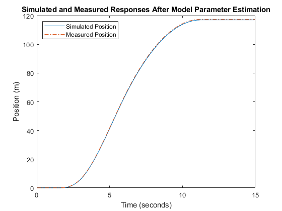
It can be seen that the model response using the estimated parameter values nicely matches the experiment output data.

plot(...
    Position.Values.Time,Position.Values.Data, ...
    Exp.OutputData.Values.Time, Exp.OutputData.Values.Data,'-.')
title('Simulated and Measured Responses After Model Parameter Estimation')
ylabel('Position (m)')
xlabel('Time (seconds)')
legend('Simulated Position','Measured Position','Location','NorthWest')

Update the Model Parameter Values

Update the model u_static and u_dynamic parameter values.

sdo.setValueInModel('sdoFriction',pOpt);

Close the model.

bdclose('sdoFriction')