Design Exploration Using Parameter Sampling (GUI)

Open Script

This example shows how to sample and explore a design space using the Sensitivity Analyzer. You explore the design of a Continuously Stirred Tank Reactor (CSTR) to minimize product concentration variation and production cost. The design must also account for the uncertainty in the temperature and concentration of the input feed to the reactor.

You explore the CSTR design by characterizing model parameters using probability distributions. You use the distributions to generate random samples and perform Monte-Carlo evaluation of the design at these sample points. You then create plots to visualize the design space and select the best design. You then use the best design as an initial guess for optimization of the design.

Continuously Stirred Tank Reactor (CSTR) Model

Continuously Stirred Tank Reactors (CSTRs) are common in the process industry. The Simulink® model, sdoCSTR, models a jacketed diabatic (i.e., non-adiabatic) tank reactor described in [1]. The CSTR is assumed to be perfectly mixed, with a single first-order exothermic and irreversible reaction, $A\rightarrow B$ . $A$ , the reactant, is converted to $B$ , the product.

In this example, you use the following two-state CSTR model, which uses basic accounting and energy conservation principles:

$\frac{d C_A}{dt} = \frac{F}{A * h}(C_{feed} - C_A)-r*C_A$

$\frac{d T}{dt} = \frac{F}{A * h}(T_{feed} - T) - \frac{H}{c_p \rho} r
-\frac{U}{c_p*\rho*h}(T - T_{cool})$

$r = k_0*e^{\frac{-E}{R*T}}$

, and $C_{feed}$ - Concentrations of A in the CSTR and in the feed [kgmol/m^3]

, $T_{feed}$ , and $T_{cool}$ - CSTR, feed, and coolant temperatures [K]

and $\rho$ - Volumetric flow rate [m^3/h] and the density of the material in the CSTR [1/m^3]

and - Height [m] and heated cross-sectional area [m^2] of the CSTR.

- Pre-exponential non-thermal factor for reaction $A\rightarrow B$ [1/h]

and - Activation energy and heat of reaction for $A\rightarrow B$ [kcal/kgmol]

- Boltzmann's gas constant [kcal/(kgmol * K)]

and - Heat capacity [kcal/K] and heat transfer coefficients [kcal/(m^2 * K * h)]

Open the Simulink model.

open_system('sdoCSTR');

CSTR Design Problem

Assume that the CSTR is cylindrical, with the coolant applied to the base of the cylinder. Tune the CSTR cross-sectional area, $A$ , and CSTR height, $h$ , to meet the following design goals:

Minimize the variation in residual concentration, . Variations in the residual concentration negatively affect the quality of the CSTR product. Minimizing the variations also improves CSTR profit.

Minimize the mean coolant temperature $T_{cool}$ . Heating or cooling the jacket coolant is expensive. Minimizing the mean coolant temperature improves CSTR profit.

The quality of the feed to the reactor can differ among suppliers. Thus, the design must allow for variations in the supply feed concentration, $C_{feed}$ , and feed temperature, $T_{feed}$ . The quality of the feed differs from supplier to supplier and also varies within each supply batch.

Specify Design Variables

Open the Sensitivity Analyzer. In the Simulink model from the Apps tab, click Sensitivity Analyzer under Control Systems. The app opens with an empty Sensitivity Analysis session.

Create a parameter set that includes the CSTR design variables A and h and the feed variation parameters FeedConc0 and FeedTemp0. You randomly generate multiple values for these parameters to evaluate the CSTR design.

In the Sensitivity Analysis tab, in the Select Parameters drop-down menu, select New.
In the dialog box, select A, FeedCon0, FeedTemp0, and h.
Click OK. An empty parameter set, ParamSet is created in the Parameter Set area of the app browser.

Specify the parameter distributions and correlations. ParamSet will be populate with parameter values selected randomly from the specified distributions:

Sample A from a uniform distribution with lower bound 0.2 m^2 and upper bound 2 m^2.
Sample h from a uniform distribution with lower bound 0.5 m and upper bound 3 m.
Sample FeedConc0 from a normal distribution with mean 10 kgmol/m^3 and standard deviation 0.5 kgmol/m^3.
Sample FeedTemp0 from a normal distribution with mean 295 K and standard deviation 3 K.
Specify FeedCon0 and FeedTemp0 as negatively correlated with covariance 0.6.

To generate 100 parameter values using the above distribution and correlation information, click Generate Values, and select Generate Random Values. For repeatability of the example reset the random number generator.

rng('default')

In the Generate Random Parameter Values dialog box, specify the following:

Set the number of samples to 100
For parameter A select Uniform distribution, set the lower bound to 0.2 and upper bound to 2.
For parameter FeedCon0 select Normal distribution, set mu to 10 and sigma to 0.5, and check cross-correlated.
For parameter FeedTemp0 select Normal distribution, set mu to 295 and sigma to 3, and check cross-correlated.
For parameter h select Uniform distribution, set the lower bound to 0.5 and upper bound to 3.
In the Correlation Matrix tab, set the FeedCon0, FeedTemp0 covariance to -0.6.
Click OK to generate the parameter values.

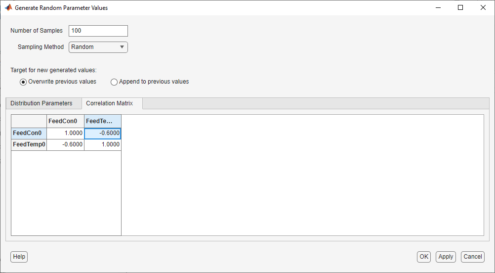
The ParamSet table is updated with the generated parameter values. Note that you can manually edit the generated parameter values in the ParamSet table.

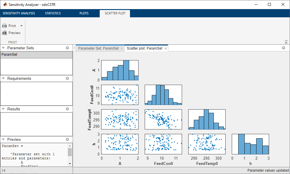
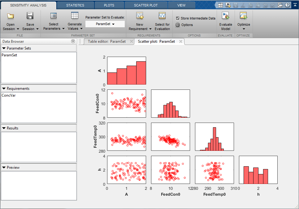
To plot the parameter set click ParamSet in the Parameter Sets area of the app browser. In the Plots tab, select Scatter Plot in the plots gallery. The plot shows the histogram of the generated parameters on the diagonal and pair-wise parameter values on the off-diagonal.

Note that due to the random number generator the specific values in the plots and tables below may differ from what you get when running the example.

Each marker on the plot represents one row of the ParamSet table, with each row being simultaneously displayed on all the plots. The correlation between FeedCon0 and FeedTemp0 can be seen on the plot.

Specify Requirements for Evaluation

The CSTR design is required to minimize the variation in residual concentration and minimize the mean coolant temperature. Select New Requirement and click Signal Property to create a requirement to minimize the residual concentration variation.

In the Create Requirement dialog box, specify the following fields:

In the Property drop-down list, select Signal Variance.
In the type drop-down list, select Minimize.
In the Select Signals area, select a logged signal to apply the requirement to. To do so click +. A Create Signal Set dialog box opens where you specify the logged signal. In the Simulink model, click the signal at the CA output of the CSTR block. The dialog box now displays this signal. Add the signal to the signal set and click OK.

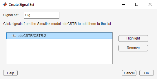
Close the Signal Property requirement dialog box by clicking the x in the upper right dialog box corner.

Close the Create Requirement dialog box. A new requirement, SignalProperty is listed in the Requirements area of the app browser

Right-click SignalProperty, select Rename; rename the requirement to ConcVar.

Select New Requirement and click Signal Property to create a requirement to minimize the coolant mean (output of block sdoCSTR/Controller) temperature.

In the Create Requirement dialog box, specify the following fields:

In the Property drop-down list, select Signal Mean.
In the Type drop-down list, select Minimize.
In the Select Signals area, add the sdoCSTR/Controller signal to the requirement.

Close the Create Requirement dialog box. A new requirement, SignalProperty is created in the Requirements area of the app browser. Rename the requirement CoolMean.

Evaluate

In the Sensitivity Analysis tab, click Select for Evaluation. By default, all requirements are selected to be evaluated. Click Evaluate Model to evaluate the ConcVar and CoolMean requirements for each row of parameter values in ParamSet. Note you can speed up evaluation by using parallel computing if you have the Parallel Computing Toolbox (TM), or by using fast restart. For more information, see "Use Parallel Computing for Sensitivity Analysis" and "use Fast Restart Mode During Sensitivity Analysis" in the Simulink Design Optimization™ documentation.

A results scatter plot showing each parameter vs each requirement is updated during model evaluation. At the end of evaluation a table with the evaluation results is created, each row in the evaluation result table contains values for A, FeedCon0, FeedTemp0, h and the resulting requirement values ConcVar and CoolMean. The evaluation results are stored in the EvalResult variable in the Results area of the app.

Analyze the Evaluation Results

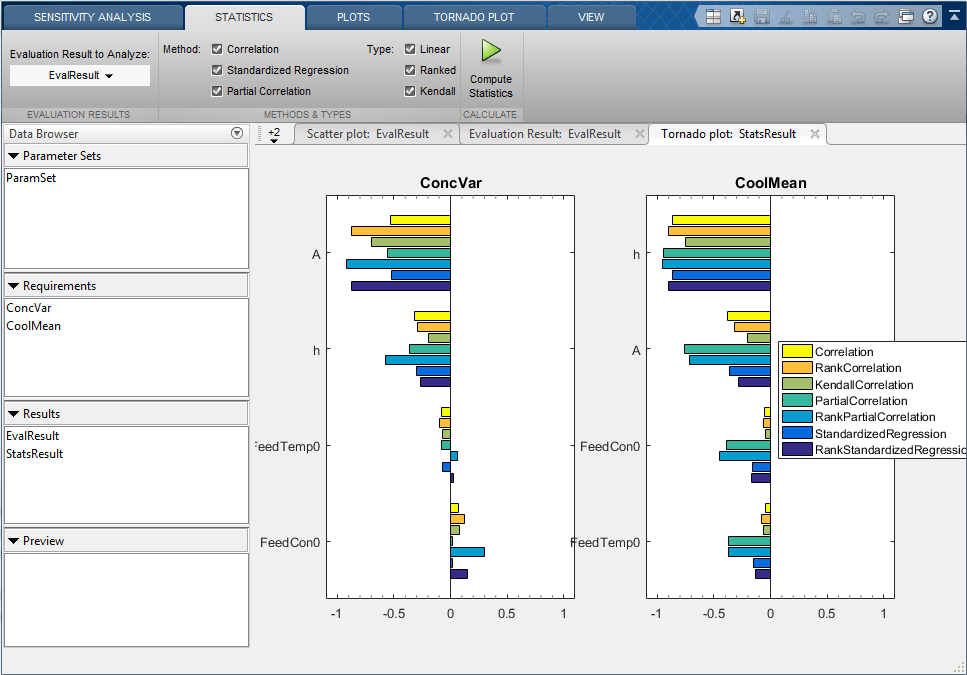
The results scatter plot for EvalResult shows that CoolMean is inversely correlated with h (increasing h decreases CoolMean) and that low values of h can result in high values for ConcVar. The plot shows that low values of A can result in high values for ConcVar, but it is not clear from the plot how A is correlated with ConcVar or CoolMean or which parameter influences ConcVar the most. To investigate further, in the Statistics tab, select all the analysis methods and types and click Compute Statistics. This performs analysis on the evaluation results and creates a tornado plot. The tornado plot shows the influence of each parameter on each requirement:

h is inversely correlated with CoolMean, and is the parameter that influences CoolMean the most.
A is inversely correlated with CoolMean.
FeedCon0 and FeedTemp0 are inversely correlated with CoolMean.
A is inversely correlated with ConcVar, and is the parameter that influences ConcVar the most.
h is inversely correlated with ConcVar.
FeedCon0 and FeedTemp0 have mixed correlation with ConVar, but have minimal correlation with ConcVar.

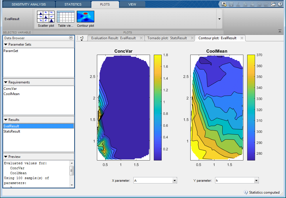
The analysis shows that choosing a large h, to reduce CoolMean and choosing a large A to reduce CoolVar would appear to be a good design choice. You can confirm this by creating a contour plot of CoolMean and CoolVar versus h and A. Select EvalResult from the Results area of the app browser, and in the Plots tab, in the plots gallery click Contour plot. On the contour plot select h for the Y parameter, note that large h medium values of A give low values for both ConcVar and CoolMean.

Choose an Initial Guess for Optimization

Sort the Evaluation Result table by decreasing h, and select a row that has low ConcVar and CoolMean values. Right-click the selected row and click Extract Parameter Values. The extracted parameter values are saved in the ParamValues variable in the Results area of the app browser. These parameter values are used as the initial guess for optimization.

Optimize

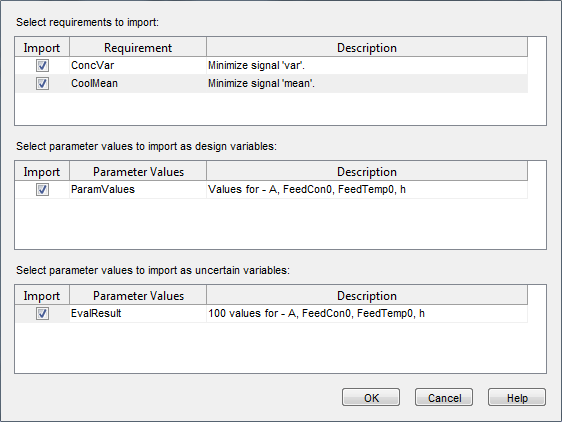
Use the data in the Sensitivity Analyzer to create an optimization problem to optimize A and h. In the Sensitivity Analysis tab click Optimize, and select Create Response Optimization Session. This opens a dialog box to import data from Sensitivity Analysis to Response Optimizer.

Select both the ConcVar and CoolMean requirements to import.
Select ParamValues to import as design variables for optimization.
Select EvalResult to import as uncertain variables to use during optimization.
Click OK to import the data to the Response Optimizer app.

Configure the Response Optimizer to optimize the CSTR design:

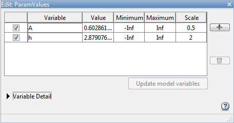
Click the pencil icon to edit the ParamValues design variable set, and remove the FeedCon0 and FeedTemp0 variables from the design variable set.

Select EvalResult as the uncertain variable set, click the pencil icon to edit EvalResult, and remove A and h from the uncertain variable set.

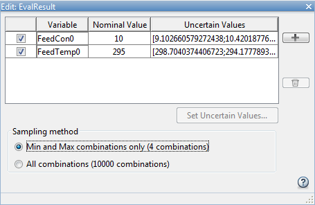
Add iteration plots to see how the variables ParamValues (A and h), and optimization requirements ConcVar and CoolMean change during optimization.

Select the variables in the Data to Plot drop-down list, and select Iteration Plot in the Add Plot drop-down list.
Click Optimize.

The optimization minimizes CoolMean and ConcVar in the presence of varying FeedCon0 and FeedTemp0.

Related Examples

To learn how to explore the CSTR design space using the sdo.evaluate command, see Design Exploration Using Parameter Sampling (Code).

References

[1] Bequette, B.W. Process Dynamics: Modeling, Analysis and Simulation. 1st ed. Upper Saddle River, NJ: Prentice Hall, 1998.

Close the model

bdclose('sdoCSTR')