Analyze Battery Impedance Using Exact Linearization

Since R2024b

This example shows how to measure the impedance of a battery designed using Simscape™ Battery™ software. You can use impedance analysis to measure the performance and characteristics of a battery. For a battery modeled using the Battery Equivalent Circuit (Simscape Battery) block, you can analyze the impedance using the linearization tools from Simulink® Control Design™ software. In this example, you linearize the model at 100% state of charge (SOC) and compare the linearization results with the transfer function that you manually derive from the equivalent circuit model. This example also shows how to use batch linearization to linearize the model at different SOC levels.

Examine Model

The example model uses a Battery Equivalent Circuit block and discharges from different SOC levels at a constant current value.

Linearize Model and Compare with Derived Transfer Function

To obtain a linear model of the Battery Equivalent Circuit block, you can use the linearize command. This example provides a Simulink model with preconfigured linear analysis points.

Open the model.

mdl_linearize = "BatteryImpedanceLinearize";
open_system(mdl_linearize);

Linearize the model at the default SOC value of 100% defined in the variable soc_ini.

io = getlinio(mdl_linearize);
linsys_soc100 = linearize(mdl_linearize,io,0.5);

For this model, the parameter values of the Battery Equivalent Circuit block describe the circuit in this image.

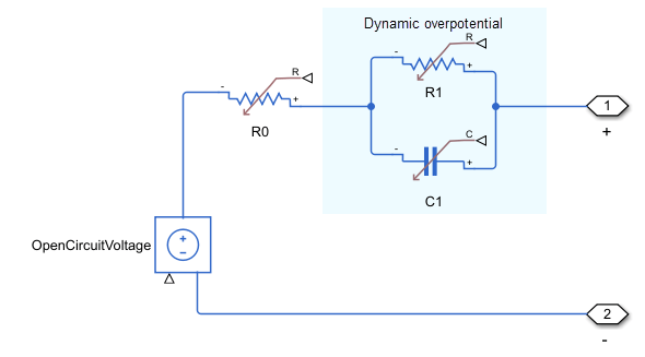
The Simulink model has one time constant that corresponds to the resistor-capacitor pair represented in the image by the R1 and C1 blocks. Based on the circuit diagram, this transfer function describes the impedance:

${\rm Z}={\mathit{R}}_0+\frac{{\mathit{R}}_{\mathit{1}}}{{\tau }_1\mathit{s}+1}$.

At an SOC level of 100%, you can manually derive the transfer function using the values defined in the block parameters.

R0 = 0.0085;
R1 = 0.017;
Tau1 = 0.39;
Z_soc100 = tf([Tau1*R0 R0+R1],[Tau1 1]);

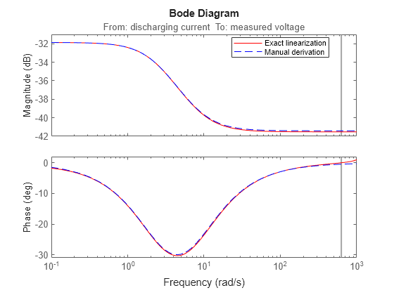
Compare the impedance results obtained from linearization and your manual derivation.

figure;
w = logspace(-1,3,100);
bode(linsys_soc100,w,"r",Z_soc100,"b--");
legend("Exact linearization","Manual derivation",Location="best");

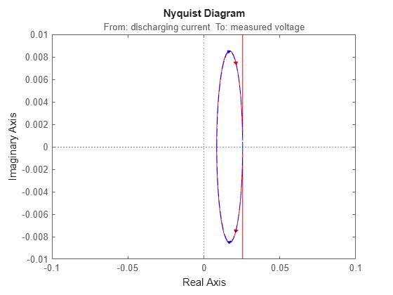
You can also compare the Nyquist response of the two models using the nyquist command.

nyquist(linsys_soc100,"r",Z_soc100,"b--")
axis([-0.1 0.1 -0.01 0.01])

Use Batch Linearization to Compare Different Levels of SOC

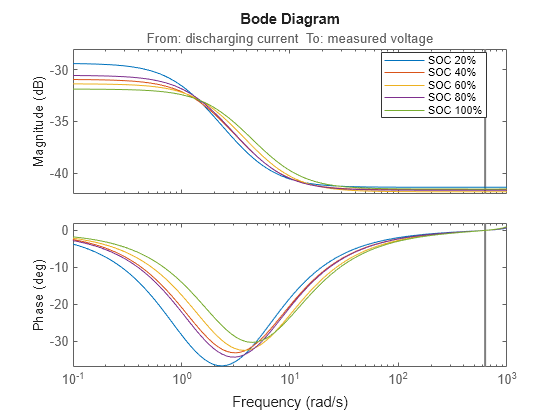
Using batch linearization, you can linearize the model at different SOC levels and compare the results. Define five SOC values from 20% to 100%.

soc_grid = 0.2:0.2:1;

Use the soc_ini variable to vary the SOC value and perform the batch linearization.

params(1).Name = "soc_ini";
params(1).Value = soc_grid;
lin_sys_soc = linearize(mdl_linearize,io,0.5,params);

The batch linearization result is an array of state-space models that correspond to the SOC values.

Plot the batch linearization results.

figure;
bodeplot(lin_sys_soc(:,:,1,1),lin_sys_soc(:,:,2,1),...
    lin_sys_soc(:,:,3,1),lin_sys_soc(:,:,4,1),...
    lin_sys_soc(:,:,5,1),w);
legend("SOC 20%","SOC 40%","SOC 60%","SOC 80%","SOC 100%",Location="best");

Create LPV Model of Battery Cell

A linear parameter-varying (LPV) system is a state-space model with dynamics that change based on time-dependent parameters called scheduling parameters. In MATLAB®, you can represent LPV models as state-space models with parameter-dependent state-space coefficients. For more information, see LTV and LPV Modeling. For this example, to construct a gridded LPV model dependent on the SOC parameter, you can use the batch linearization results from the previous section.

To construct the gridded LPV model, use the ssInterpolant function.

lpv_sys_soc = ssInterpolant(lin_sys_soc,'spline');

An LPV model simplifies battery cell behavior analysis due to its lower model complexity. For example, you can resample the LPV model using finer grids of SOC values without performing linearization again. Sample the LPV model at a 5% step instead of the 20% step used in batch linearization. This returns a time-invariant state-space model array where each model corresponds to the SOC value at that index.

soc_fine_grid = 0.2:0.05:1;
ssArray = psample(lpv_sys_soc,[],soc_fine_grid);
figure; 
bode(ssArray,w);

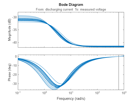
This model captures the behavior at different SOC levels and greatly reduces battery cell model complexity. Therefore, such LPV models provide low-complexity approximations of high-fidelity models that support fast simulation and analysis.

close_system(mdl_linearize);