Variable Step Solvers in Simulink

Variable-step solvers vary the step size during the simulation, reducing the step size to increase accuracy when model states are changing rapidly and increasing the step size to avoid taking unnecessary steps when model states are changing slowly. Computing the step size adds to the computational overhead at each step but can reduce the total number of steps, and hence simulation time, required to maintain a specified level of accuracy for models with rapidly changing or piecewise continuous states.

When you set the Type control of the Solver configuration pane to Variable-step, the Solver control allows you to choose one of the variable-step solvers. As with fixed-step solvers, the set of variable-step solvers comprises a discrete solver and a collection of continuous solvers. However, unlike the fixed-step solvers, the step size varies dynamically based on the local error.

The choice between the two types of variable-step solvers depends on whether the blocks in your model define states and, if so, the type of states that they define. If your model defines no states or defines only discrete states, select the discrete solver. If the model has continuous states, the continuous solvers use numerical integration to compute the values of the continuous states at the next time step.

Note

If a model has no states or only discrete states, Simulink^® uses the discrete solver to simulate the model even if you specify a continuous solver.

Variable-Step Discrete Solver

Use the variable-step discrete solver when your model does not contain continuous states. For such models, the variable-step discrete solver reduces its step size in order to capture model events such as zero-crossings, and increases the step size when it is possible to improve simulation performance.

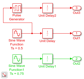
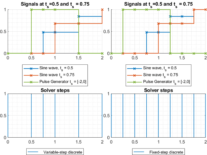
The model shown in the figure contains two discrete sine wave signals at 0.5 and 0.75 sample times. The graphs below show the signals in the model along with the solver steps for the variable-step discrete and the fixed-step discrete solvers respectively. You can see that the variable-step solver only takes the steps needed to record the output signal from each block. On the other hand, the fixed-step solver will need to simulate with a fixed-step size—or fundamental sample time—of 0.25 to record all the signals, thus taking more steps overall.

Variable-Step Continuous Solvers

Variable-step solvers dynamically vary the step size during the simulation. Each of these solvers increases or reduces the step size using its local error control to achieve the tolerances that you specify. Computing the step size at each time step adds to the computational overhead. However, it can reduce the total number of steps, and the simulation time required to maintain a specified level of accuracy.

You can further categorize the variable-step continuous solvers as one-step or multistep, single-order or variable-order, and explicit or implicit. See One-Step Versus Multistep Continuous Solvers for more information.

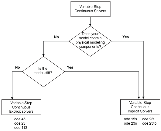
Variable-Step Continuous Explicit Solvers

The variable-step explicit solvers are designed for nonstiff problems. Simulink provides four such solvers:

ode45
ode23
ode113
odeN

ODE Solver	One-Step Method	Multistep Method	Order of Accuracy	Method
`ode45`	X		Medium	Runge-Kutta, Dormand-Prince (4,5) pair
`ode23`	X		Low	Runge-Kutta (2,3) pair of Bogacki & Shampine
`ode113`		X	Variable, Low to High	PECE Implementation of Adams-Bashforth-Moulton
`odeN`	X		See Order of Accuracy in Fixed-Step Continuous Explicit Solvers	See Integration Technique in Fixed-Step Continuous Explicit Solvers

ODE Solver	When to Use
ode45	In general, the `ode45` solver is the best to apply as a first try for most problems. The Runge-Kutta (4,5) solver is a fifth-order method that performs a fourth-order estimate of the error. This solver also uses a fourth-order interpolant, which allows for event location and smoother plots. If the `ode45` is computationally slow, the problem may be stiff and thus require an implicit solver.
ode113	For problems with stringent error tolerances or for computationally intensive problems, the Adams-Bashforth-Moulton PECE solver can be more efficient than `ode45`.
ode23	The `ode23` can be more efficient than the `ode45` solver at crude error tolerances and in the presence of mild stiffness. This solver provides accurate solutions by applying a cubic Hermite interpolation to the values and slopes computed at the ends of a step.
odeN	The `odeN` solver uses a nonadaptive Runge-Kutta integration whose order is determined by the Solver order parameter. `odeN` uses a fixed step size determined by the Max step size parameter, but the step size can be reduced to capture certain solver events, such as zero-crossings and discrete sample hits.

Note

Select the odeN solver when simulation speed is important, for example, when

The model contains lots of zero-crossings and/or solver resets
The Solver Profiler does not detect any failed steps when profiling the model

Variable-Step Continuous Implicit Solvers

If your problem is stiff, try using one of the variable-step implicit solvers:

ode15s
ode23s
ode23t
ode23tb

ODE Solver	One-Step Method	Multistep Method	Order of Accuracy	Solver Reset Method	Max. Order	Method
`ode15s`		X	Variable, low to medium	X	X	Numerical Differentiation Formulas (NDFs)
`ode23s`	X		Low			Second-order, modified Rosenbrock formula
`ode23t`	X		Low	X		Trapezoidal rule using interpolant
`ode23tb`	X		Low	X		TR-BDF2

Solver Reset Method

For ode15s, ode23t, and ode23tb a drop-down menu for the Solver reset method appears in the Solver details section of the Configuration pane. This parameter controls how the solver treats a reset caused, for example, by a zero-crossing detection. The options allowed are Fast and Robust. Fast specifies that the solver does not recompute the Jacobian for a solver reset, whereas Robust specifies that the solver does. Consequently, the Fast setting is computationally faster but it may use a small step size in certain cases. To test for such cases, run the simulation with each setting and compare the results. If there is no difference in the results, you can safely use the Fast setting and save time. If the results differ significantly, try reducing the step size for the fast simulation.

Maximum Order

For the ode15s solver, you can choose the maximum order of the numerical differentiation formulas (NDFs) that the solver applies. Since the ode15s uses first- through fifth-order formulas, the Maximum order parameter allows you to choose orders 1 through 5. For a stiff problem, you may want to start with order 2.

Tips for Choosing a Variable-Step Implicit Solver

The following table provides tips for the application of variable-step implicit solvers. For an example comparing the behavior of these solvers, see Explore Variable-Step Solvers with Stiff Model.

ODE Solver	Tips on When to Use
ode15s	`ode15s` is a variable-order solver based on the numerical differentiation formulas (NDFs). NDFs are related to, but are more efficient than the backward differentiation formulas (BDFs), which are also known as Gear's method. The `ode15s` solver numerically generates the Jacobian matrices. If you suspect that a problem is stiff, or if `ode45` failed or was highly inefficient, try `ode15s`. As a rule, start by limiting the maximum order of the NDFs to 2.
ode23s	`ode23s` is based on a modified Rosenbrock formula of order 2. Because it is a one-step solver, it can be more efficient than `ode15s` at crude tolerances. Like `ode15s`, `ode23s` numerically generates the Jacobian matrix for you. However, it can solve certain kinds of stiff problems for which `ode15s` is not effective.
ode23t	The `ode23t` solver is an implementation of the trapezoidal rule using a “free” interpolant. Use this solver if your model is only moderately stiff and you need a solution without numerical damping. (Energy is not dissipated when you model oscillatory motion.)
ode23tb	`ode23tb` is an implementation of TR-BDF2, an implicit Runge-Kutta formula with two stages. The first stage is a trapezoidal rule step while the second stage uses a backward differentiation formula of order 2. By construction, the method uses the same iteration matrix in evaluating both stages. Like `ode23s`, this solver can be more efficient than `ode15s` at crude tolerances.

Note

For a stiff problem, solutions can change on a time scale that is very small as compared to the interval of integration, while the solution of interest changes on a much longer time scale. Methods that are not designed for stiff problems are ineffective on intervals where the solution changes slowly because these methods use time steps small enough to resolve the fastest possible change. For more information, see Shampine, L. F., Numerical Solution of Ordinary Differential Equations, Chapman & Hall, 1994.

Error Tolerances for Variable-Step Solvers

Local Error

The variable-step solvers use standard control techniques to monitor the local error at each time step. During each time step, the solvers compute the state values at the end of the step and determine the local error—the estimated error of these state values. They then compare the local error to the acceptable error, which is a function of both the relative tolerance (rtol) and the absolute tolerance (atol). If the local error is greater than the acceptable error for any one state, the solver reduces the step size and tries again.

Relative tolerance measures the error relative to the size of each state. The relative tolerance represents a percentage of the state value. The default, 1e-3, means that the computed state is accurate to within 0.1%.
Absolute tolerance is a threshold error value. This tolerance represents the acceptable error as the value of the measured state approaches zero.
The solvers require the error for the ith state, e_i, to satisfy:

$e_{i} \leq \max (r t o l \times | x_{i} |, a t o l_{i}) .$

The following figure shows a plot of a state and the regions in which the relative tolerance and the absolute tolerance determine the acceptable error.

Absolute Tolerances

Your model has a global absolute tolerance that you can set on the Solver pane of the Configuration Parameters dialog box. This tolerance applies to all states in the model. You can specify auto or a real scalar. If you specify auto (the default), Simulink initially sets the absolute tolerance for each state based on the relative tolerance. If the relative tolerance is larger 1e-3, abstol is initialized at 1e-6. However, for reltol smaller than 1e-3, abstol for the state is initialized at reltol * 1e-3. As the simulation progresses, the absolute tolerance for each state resets to the maximum value that the state has assumed so far, times the relative tolerance for that state. Thus, if a state changes from 0 to 1 and reltol is 1e-3, abstol initializes at 1e-6 and by the end of the simulation reaches 1e-3 also. If a state goes from 0 to 1000, then abstol changes to 1.

Now, if the state changes from 0 to 1 and reltol is set at 1e-4, then abstol initializes at 1e-7 and by the end of the simulation reaches a value of 1e-4.

If the computed initial value for the absolute tolerance is not suitable, you can determine an appropriate value yourself. You might have to run a simulation more than once to determine an appropriate value for the absolute tolerance. You can also specify if the absolute tolerance should adapt similarly to its auto setting by enabling or disabling the AutoScaleAbsTol parameter. For more information, see Auto scale absolute tolerance.

Several blocks allow you to specify absolute tolerance values for solving the model states that they compute or that determine their output:

The absolute tolerance values that you specify for these blocks override the global settings in the Configuration Parameters dialog box. You might want to override the global setting if, for example, the global setting does not provide sufficient error control for all of your model states because they vary widely in magnitude. You can set the block absolute tolerance to:

auto
–1 (same as auto)
positive scalar
real vector (having a dimension equal to the number of corresponding continuous states in the block)

Tips

If you do choose to set the absolute tolerance, keep in mind that too low of a value causes the solver to take too many steps in the vicinity of near-zero state values. As a result, the simulation is slower.

On the other hand, if you set the absolute tolerance too high, your results can be inaccurate as one or more continuous states in your model approach zero.

Once the simulation is complete, you can verify the accuracy of your results by reducing the absolute tolerance and running the simulation again. If the results of these two simulations are satisfactorily close, then you can feel confident about their accuracy.