Use local solver when referencing model

Option to use local solver to solve referenced model as separate system of equations

Since R2022a

Model Configuration Pane: Model Referencing

Description

The Use local solver when referencing model configuration parameter specifies how the software solves the system implemented by a referenced model. When you select this parameter, the software solves the referenced model as a separate set of differential equations using the solver that the current referenced model specifies for the Solver configuration parameter.

While the top solver can be a fixed-step or variable-step solver, the local solver must be a fixed-step solver. Specify the fixed step size for the local solver using the Fixed-step size (fundamental sample time) configuration parameter of the referenced model.

Using a local solver can facilitate system composition and integration. When you use local solvers, you can solve referenced models in system-level simulations using the same solver and step size used to design and test each model in isolation. Using local solvers can also reduce the amount of configuration adjustments you need to make to configuration parameters in referenced models while integrating the model into a larger system.

For some systems, using a local solver can improve simulation performance by allowing you to choose a solver that is more appropriate to solve the system in the referenced model or by reducing the number of redundant calculations in systems that have a wide range of dynamics among components.

For an example, see Improve Simulation Performance by Using Local Solvers.

For more information about local solvers, see Use Local Solvers in Referenced Models.

Set Configuration Parameter for Referenced Model

In a model reference hierarchy, how you open the Configuration Parameters dialog box determines whether you edit the configuration parameter for the top model in the current model hierarchy or the current referenced model.

• Top model in the current model hierarchy — In the Simulink^® Toolstrip, on the Modeling tab, click Model Settings.

• Current referenced model — In the Simulink Toolstrip, on the Modeling tab, click the Model Settings button arrow. Then, in the Referenced Model section, select Model Settings.

Alternatively, open the referenced model as a top model. Then, in the Simulink Toolstrip, on the Modeling tab, click Model Settings.

Settings

off (default) | on

on

The software uses a local solver to solve the referenced model as a separate set of differential equations. Specify the local solver using the Solver configuration parameter of the referenced model.

off

The software solves the referenced model as part of the parent system using the parent solver.

Examples

Configure Local Solver for Component with Fast Dynamics

Open the model SecondOrderSystemTop. The model contains a Ramp block that provides the input signal for a Model block that references a model of a second-order system. The Model block output signal connects to an Outport block.

topmdl = "SecondOrderSystemTop";
open_system(topmdl)

To navigate inside the referenced model, double-click the Model block. Alternatively, create a Simulink.BlockPath object for the Model block and use the open function to open the referenced model in the context of the model hierarchy.

mdlblkpath = Simulink.BlockPath(topmdl + "/Model");
open(mdlblkpath)

The referenced model implements the second-order system using a Transfer Fcn block and contains a Step block that models a change or disturbance to the system.

The system transfer function is specified in the Transfer Fcn block using two model workspace variables, wn and z, which represent the natural frequency of the system, in radians per second, and the system damping coefficient.

Configure the system with a natural frequency of 100 radians per second by specifying the value of the variable wn as 100 in the model workspace.

refmdl = "SecondOrderSystem";
mdlwksp = get_param(refmdl,"ModelWorkspace");
assignin(mdlwksp,"wn",100)

Configure the referenced model to use a local solver with a step size of 0.01 seconds. You can configure the settings for the referenced model from the top model using the Property Inspector or the Block Parameters dialog box.

1. Open the Property Inspector. On the Modeling tab, expand the Design section and select Property Inspector, or press Ctrl+Shift+I.

2. To open the Configuration Parameters dialog box for the referenced model, select the Model block. Then, in the Property Inspector, expand the Solver section and click the hyperlink next to the Use local solver parameter.

3. Configure the model to use a local solver when referenced in a model hierarchy. In the Configuration Parameters dialog box, on the Model Referencing pane, select Use local solver when referencing model.

4. Select the fixed-step ode3 as the local solver. On the Solver pane, from the Type list, select Fixed-step. Then, from the Solver list, select ode3 (Bogacki-Shampine).

5. Set the local solver step size to 0.01 seconds. On the Solver pane, expand Solver details. Then, in the Fixed-step size (fundamental sample time) box, enter 0.01.

6. Click OK.

Alternatively, use the set_param function to configure the parameters.

set_param(refmdl,UseModelRefSolver="on",...
    SolverType="Fixed-Step",Solver="ode3",FixedStep="0.01")

In the top model, the Model block indicates the local solver you specify.

Specify the communication step size for the model reference. The communication step size specifies when the parent and local solvers exchange data and is registered as a discrete sample time in the top model.

The Ramp block in the top model has a slope of 0.2, and the top solver uses a step size of 0.2 seconds. Because the input signal from the top model changes slowly compared to the dynamics of the second-order system, the communication step size can be much larger than the local solver step size without significant effect on the accuracy of the simulation results.

Specify the communication step size as 0.4 seconds. Select the Model block. Then, in the Property Inspector, under Solver, in the Communication step size box, enter 0.4.

Alternatively, use the set_param function to set the CommunicationStepSize parameter.

set_param(topmdl + "/Model",CommunicationStepSize="0.4")

Simulate the model, using the local solver to compute the response of the second-order system.

out = sim(topmdl);

To view the simulation results, open the Simulation Data Inspector. On the Simulation tab, under Review Results, click Data Inspector. Alternatively, call the Simulink.sdi.view function.

Simulink.sdi.view

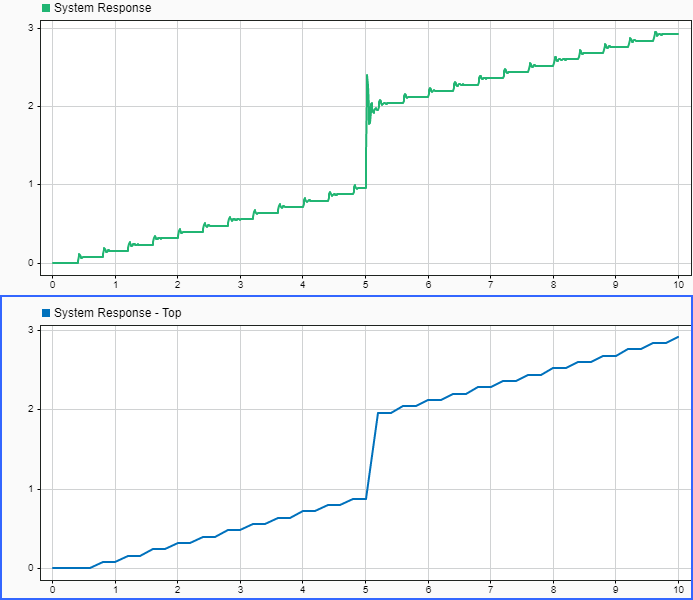
Plot the signals named System Response and System Response - Top on separate subplots. Alternatively, use the Simulink.sdi.loadView function to load the view named FastSecondOrderSystem, which was created for this example.

Simulink.sdi.loadView("FastSecondOrderSystem.mldatx");

The System Response and System Response - Top signals are the same signal, logged in different locations. The System Response signal is logged inside the referenced model at a rate determined by the local solver step size. The System Response - Top signal is logged by the Outport block in the top model at a rate determined by the top solver step size. Because the local solver step size is much smaller than the top solver step size, the System Response signal captures the system response to the change in the input signal when the Step block output value changes with higher fidelity.

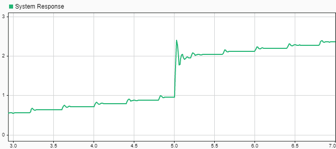
In the System Response signal, you can see the effect of the local solver interpolating the input signal with a zero-order hold between each communication step. If you zoom on the time axis around 5 seconds, you can see the oscillations in the system response to the step.

Configure Local Solver for Component with Slow Dynamics

Open the model SecondOrderSystemTop. The model contains a Ramp block that provides the input signal for a Model block that references a model of a second-order system. The Model block output signal connects to an Outport block.

topmdl = "SecondOrderSystemTop";
open_system(topmdl)

To navigate inside the referenced model, double-click the Model block. Alternatively, create a Simulink.BlockPath object for the Model block and use the open function to open the referenced model in the context of the model hierarchy.

mdlblkpath = Simulink.BlockPath(topmdl + "/Model");
open(mdlblkpath)

The referenced model implements the second-order system using a Transfer Fcn block and contains a Step block that models a change or disturbance to the system.

The system transfer function is specified in the Transfer Fcn block using two model workspace variables, wn and z, which represent the natural frequency of the system, in radians per second, and the system damping coefficient.

Configure the system with a natural frequency of 1 radian per second by specifying the value of the variable wn as 1 in the model workspace.

refmdl = "SecondOrderSystem";
mdlwksp = get_param(refmdl,"ModelWorkspace");
assignin(mdlwksp,"wn",1)

Configure the referenced model to use a local solver with a step size of 0.4 seconds. You can configure the settings for the referenced model from the top model using the Property Inspector or the Block Parameters dialog box.

1. Open the Property Inspector. On the Modeling tab, expand the Design section and select Property Inspector, or press Ctrl+Shift+I.

2. To open the Configuration Parameters dialog box for the referenced model, select the Model block. Then, in the Property Inspector, expand the Solver section and click the hyperlink next to the Use local solver parameter.

3. Configure the model to use a local solver when referenced in a model hierarchy. In the Configuration Parameters dialog box, on the Model Referencing pane, select Use local solver when referencing model.

4. Select the fixed-step ode3 as the local solver. On the Solver pane, from the Type list, select Fixed-step. Then, from the Solver list, select ode3 (Bogacki-Shampine).

5. Set the local solver step size to 0.4 seconds. On the Solver pane, expand Solver details. Then, in the Fixed-step size (fundamental sample time) box, enter 0.4.

6. Click OK.

Alternatively, use the set_param function to configure the parameters.

set_param(refmdl,UseModelRefSolver="on",...
    SolverType="Fixed-Step",Solver="ode3",FixedStep="0.4")

In the top model, the Model block indicates the local solver you specify.

When the local solver step size is larger than the parent solver step size, inherit the communication step size by specifying the Communication step size parameter as -1. The communication step size specifies when the parent solver and local solver exchange data and is registered as a discrete sample time in the parent model.

set_param(topmdl + "/Model",CommunicationStepSize="-1")

Simulate the model, using the local solver to compute the response of the second-order system.

out = sim(topmdl,StopTime="20");

To view the simulation results, open the Simulation Data Inspector. On the Simulation tab, under Review Results, click Data Inspector. Alternatively, call the Simulink.sdi.view function.

Simulink.sdi.view

Plot the signals named System Response and System Response - Top on separate subplots. Alternatively, use the Simulink.sdi.loadView function to load the view named SlowSecondOrderSystem, which was created for this example.

Simulink.sdi.loadView("SlowSecondOrderSystem.mldatx");

The System Response and System Response - Top signals are the same signal, logged in different locations. The System Response signal is logged inside the referenced model at a rate determined by the local solver step size. The System Response - Top signal is logged by the Outport block in the top model at a rate determined by the top solver step size. Fewer data points are logged for the System Response signal because the local solver step size is larger than the parent solver step size.

Tips

• You can use Model block parameters to specify:

  • The communication step size, which specifies the rate at which the local and parent solvers exchange data

  • How the local solver extrapolates inputs from the parent solver

  • How the local solver interpolates state or output values to provide output signal values to the parent solver

• Before R2024a: When the top solver is a fixed-step solver, the step size for the local solver must be an integer multiple of the parent solver step size.

Recommended Settings

Application	Setting
Debugging	off
Traceability	No impact
Efficiency	No recommendation
Safety precaution	No impact

Programmatic Use

Parameter: UseModelRefSolver

Value: "on" | "off"

Default: "off"

Version History

Introduced in R2022a

R2024b: Improved sample time propagation for output ports of model references that use local solvers

Model blocks that reference models configured to use local solvers now propagate a discrete sample time to the block output ports if the local solver uses zero-order hold output signal handling. The Communication step size parameter of the Model block defines the discrete sample time propagated to the block output ports. In previous releases, the Model block propagated the sample time of the port in the referenced model to the block output ports.

This change to sample time propagation:

• Simplifies the interactions between the parent solver and local solver

• More clearly reflects the effect of the zero-order hold output signal handling in the context of the parent model

• Reduces the number of parent solver resets

In some cases, the change to sample time propagation causes warnings about sample time discrepancies or collisions. For example, when a Model block output port that now has a discrete sample time drives the input port of another model reference, the software issues a warning if the sample time of the input port in the referenced model does not match the sample time of the input signal in the top model. For more information, see Improve Simulation Performance Using Performance Advisor.

In most cases, this change does not affect numerical results and only results in fewer or different points in logged data for the Model block output signals. The table summarizes the impact of this change for different local solver configurations.

Local Solver Step Size	Output signal handling Parameter Value	Effect of Sample Time Propagation Change
Local solver step size less than communication step size	Zero-order hold	Model block output ports have a discrete sample time defined by the Communication step size parameter of the block. The change in sample time does not affect the numerical results of the simulation but can result in different or fewer data points in logged data for Model block output signals in the top model.
	Auto Only zero-order hold output signal handling is supported.
Local solver step size equal to communication step size	Auto	No change to sample time propagation.
	Use solver interpolant
	Zero-order hold	Model block output ports have a discrete sample time defined by the Communication step size parameter of the block. The change in sample time can result in different or fewer data points in logged data for Model block output signals in the top model. In rare cases, the change in sample time can affect numerical results as a result of: Applying the zero-order hold to output signals that do not depend on continuous states in the referenced model Performing fewer parent solver resets

R2024a: Use local solver for components with faster dynamics

You can use local solvers for system components with faster dynamics by specifying a local step size that is smaller than the parent solver step size. The new Communication step size parameter specifies the discrete rate for communication between the parent and local solver. The communication step size is registered as a discrete rate in the parent model instead of the local solver step size.

R2024a: New default Output signal handling parameter value and improved behavior when Input signal handling parameter value is Auto

The default value of the Output signal handling parameter is the new value Auto. When the Output signal handling parameter value is Auto, the software determines the method to use to interpolate continuous state or input signal values to the parent solver simulation time based on how the local step size compares to the communication step size. In previous releases, the local step size had to be greater than or equal to the parent solver step size, and the Auto option did not exist.

When the Input signal handling parameter value is Auto, the software now determines how to extrapolate continuous derivative or input signal values to the local simulation time based on the model structure and how the local step size compares to the communication step size. In previous releases, the software did not consider the model structure when selecting the interpolation method. Considering how the local step size compares to the communication step size was also not relevant because the Communication step size parameter did not exist.

R2024a: Use local solver for model that contains blocks with wrapped states

You can configure a model that contains one or more blocks with wrapped states to use a local solver when referenced in a model hierarchy. Wrapping states can improve numerical stability for systems with cyclical state values and allows the state value to wrap to the start of the cycle without resetting the solver, which can slow simulation performance.

For example, you can model the angular position of a wheel as having a value that is always between 0 and 2π. When the wheel rotates beyond an angular position of 2π, the angular position wraps back to 0 rather than continually increasing.

R2023a: Use local solver for model reference at any location in model hierarchy

Model blocks at any location in a model hierarchy can use a local solver, including Model blocks inside referenced models that use local solvers.

R2022b: Local solver support for accelerator and rapid accelerator simulation

Accelerator and rapid accelerator mode support simulating model reference hierarchies that use local solvers.