Hard Stops in the Position-Based Translational Domain

This example shows how to configure hard stop blocks in several simple position-based mechanical translational models and interpret the model behavior. This example describes how to model systems with upper and lower bounds, choose a hard stop model parameterization, set initial targets for variables, and interpret the logged forces.

Ball Bouncing On the Ground

Open the model ConfiguringHardStopsBallBouncingOnGround.

open_system('ConfiguringHardStopsBallBouncingOnGround');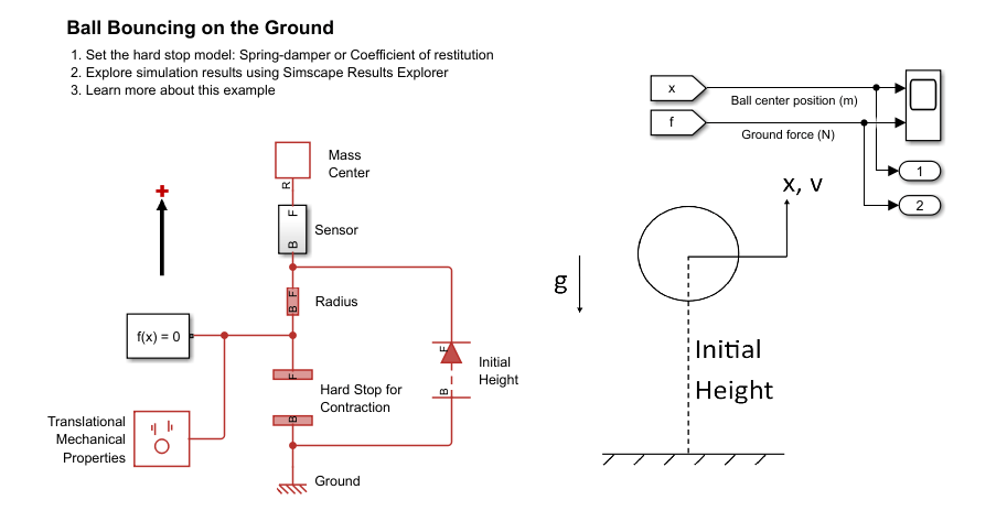

The model represents a ball that bounces on the ground, traveling in the vertical direction. Gravity acts downward, the ball has a mass of 0.5 kg and radius of 15 cm. In this scenario, the ball has an initial height of 8 m above the ground.

In the model, the entire ball mass is concentrated at a single point, labeled Mass Center. The Hard Stop for Contraction block models the contact between the ball and ground. A translational mechanical properties block specifies the network rail as pointing upwards.

The Initial Height block sets the initial distance between the ball center and ground. The Initial Height block has a high priority target distance of 8 m between the ball center and ground. The Mass Center block has a high priority target of 0 m/s for its initial velocity. These two high priority targets fully specify the model initial conditions, so all other variable targets have priorities of none.

Open the Sensor subsystem.

open_system('ConfiguringHardStopsBallBouncingOnGround/Sensor');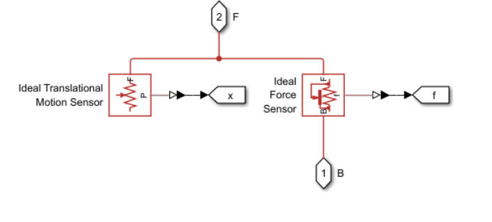

The Sensor subsystem senses the absolute position of the ball center and the force of the ground acting on the ball. The Ideal Force Sensor senses force flowing from port B to port F, meaning it senses the force of the system at port B acting on the system at port F. The sensor measures a positive force when port B exerts a positive force on port F, which is equivalent to a state of compression. The sensor measures a negative force when port B exerts a negative force on port F, which is equivalent to a state of tension. Keeping in line with the position-based mechanical translational force conventions, the sensor B and F ports align with the subsystem B and F ports and the network's global positive direction.

Open the Scope and simulate the model.

open_system('ConfiguringHardStopsBallBouncingOnGround');
open_system('ConfiguringHardStopsBallBouncingOnGround/Scope');
sim('ConfiguringHardStopsBallBouncingOnGround');

The ball starts at a position of 8 m and falls towards the ground. The ball bounces multiple times, losing energy on each collision. When the ball hits the ground, the ground imparts a large impulse on the ball in the upward direction.

Ball Bouncing Between Two Walls

Open the model ConfiguringHardStopsBallBouncingBetweenWalls.

open_system('ConfiguringHardStopsBallBouncingBetweenWalls');

The model represents a ball that bounces between two walls, traveling in the horizontal direction. The ball has a mass of 0.5 kg and radius of 15 cm. The walls are spaced 10 m apart. The ball is initially in the middle of the gap between the walls and has a velocity of 10 m/s.

In the model, the entire ball mass is concentrated at a single point, labeled Mass Center. Spacer blocks named Left Radius and Right Radius model fixed radial distances on either side of the Mass Center. The Mass Center itself has the parameter Distance between ports set to 0 m. Setting the Distance between ports to zero allows the Ideal Translational Motion Sensor attached the the Mass Center B port to output the position of the mass center. Both contact points between the ball and walls are modeled using hard stops for contraction. The point where the ball leftmost point impacts the left wall is modeled using the Left Hard Stop. Port B of the Left Hard Stop is connected to the stationary World block, so it does not move and has a position of 0 m. The point where the ball rightmost point impacts the right wall is modeled using the Right Hard Stop. Port F of the Right Hard Stop is stationary because it is connected to a Spacer block that is connected to the World block. The Spacer block sets the 10 m distance between the walls. A Translational Mechanical Properties block specifies the rail inclination as horizontal (0 degrees).

The Initial Spacer block sets the initial distance between the ball center and right wall. The Initial Spacer block has a high priority target length of 5 m. The Mass Center has a high priority target of 10 m/s for its initial velocity. These two high priority targets fully specify the model initial conditions, so all other variable targets have priorities of none.

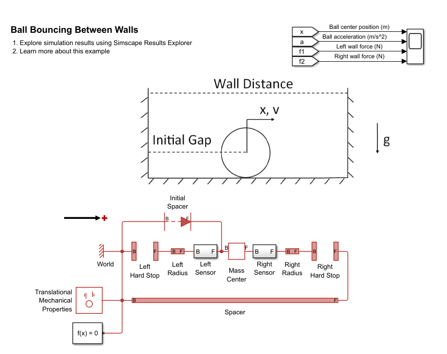
The Left Sensor subsystem contains the Ideal Translational Motion Sensor for measuring the ball center position and acceleration and an Ideal Force Sensor for measuring impacts between the ball and left wall. The Ideal Force Sensor B and F ports are aligned with the rail's positive direction. The Right Sensor subsystem contains an Ideal Force Sensor for measuring impacts between the ball and right wall.

open_system('ConfiguringHardStopsBallBouncingBetweenWalls/Left Sensor');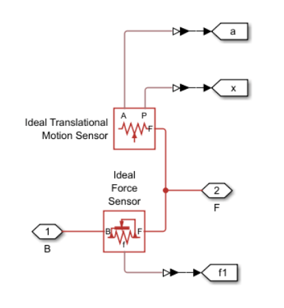

Open the Scope and simulate the model.

open_system('ConfiguringHardStopsBallBouncingBetweenWalls');
open_system('ConfiguringHardStopsBallBouncingBetweenWalls/Scope');
sim('ConfiguringHardStopsBallBouncingBetweenWalls');

The ball starts at a position of 5 m and travels in the positive direction toward the right wall. When the ball hits the right wall, it experiences a large acceleration in the negative direction as it rapidly reverses direction. The ball then bounces between the walls, losing energy after each bounce. As the ball hits each wall, the corresponding force sensor measures a large positive force, corresponding to a hard stop in a state of compression. While the hard stop that is engaged undergoes a state of compression, the other hard stop is disengaged and registers zero force. The mass absorbs all of the hard stop force.

When the ball impacts the right wall, the Right Hard Stop imparts a large negative force on the ball to generate the large negative acceleration. The figure below depicts the physical view and force flow during the impact. Force flows out of the Mass Center, corresponding to negative acceleration and negative logged force, f. Force flows from port B to port F in the Right Sensor, Right Radius, and Right Hard Stop, corresponding to states of compression and positive logged force, f, in the two-port blocks. Force flows from port F to port B in the Spacer block, corresponding to a a state of tension and negative logged force, f, in the Spacer block. Force flows into the World block, corresponding to the World block providing a negative force to the Spacer block that prevents motion in the positive direction. Zero force flows through the Left Hard Stop, Left Radius, and Left Sensor because the World and Mass Center blocks fully absorb the force.

The figure below shows the physical view and schematic view force flow during a collision with the left wall. Force flows from port B to port F in the Left Hard Stop, Left Radius, and Left Sensor, corresponding to states of compression and positive logged force, f. Force flows into the Mass Center, corresponding to the mass accelerating in the positive direction. Force flows out of the World block, corresponding to the World block preventing the Left Hard Stop B port from moving in the negative direction. The rest of the position-based translational network has zero force flowing through it, corresponding to the World block and Mass Center block fully absorbing all of the force.

Light Cable Between Two Masses

Open the model ConfiguringHardStopsCableBetweenMasses.

open_system('ConfiguringHardStopsCableBetweenMasses');

The model represents two masses that slide on a frictionless surface and are connected by a light cable. The right mass initially has a velocity of 2 m/s while the left mass is motionless. As the right mass slides to the right, the cable goes taut, snapping the left mass into motion and slowing down the right mass. The left mass travels faster than the right mass, causing the masses to collide with each other. When the left mass collides with the right mass, the left mass loses speed while the right mass gains speed. Alternating cycles of the cable going taut and the masses colliding occur as the masses continue to travel in the positive direction. The cable has a length of 1 m. The masses are modeled as point masses without any length.

In the model, the light cable is modeled by the Hard Stop for Extension block. The contact between the masses is modeled by the Hard Stop for Contraction block. An Initial Spacer block sets the initial position of Mass1 to 0 m. The Hard Stop for Extension has a high priority Gap length of 0.5 m. Mass1 has a high priority target velocity of 0 m/s while Mass2 has a high priority target velocity of 2 m/s. These high priority targets fully specify the model initial conditions, so all other variable targets have priorities of none.

Open the Sensor subsystem.

open_system('ConfiguringHardStopsCableBetweenMasses/Sensor1');

The Sensor1 subsystem senses the absolute position of Mass1 and the force flowing from Mass1 to the rest of the system. Force flowing from Mass1 to the rest of the system is equivalent to the force flowing into Mass2, due to this schematic topography.

Open the Scope and simulate the model.

open_system('ConfiguringHardStopsCableBetweenMasses');
open_system('ConfiguringHardStopsCableBetweenMasses/Scope');
sim('ConfiguringHardStopsCableBetweenMasses');

When the simulation starts, Mass1 is at rest with a position of 0 m. Mass2 has a positive velocity and position of +0.5 m relative to Mass1. When Mass2 has a position of 1 m relative to Mass1, the taut cable causes an impulse force between the masses. During the impulse, the force flowing from Mass1 to Mass2 has a negative sign, indicating that the system in between the two masses is in a state of tension. In a state of tension, the Hard Stop for Extension exerts a positive force on Mass1 (a force that accelerates Mass1 in the positive direction) and a negative force on Mass2 (a force that accelerates Mass2 in the negative direction).

At a simulation time of nearly 1 second, the masses collide. The Ideal Force Sensor measures a positive impulse force, indicating that the system in between the two masses is in a state of compression. In a state of compression, the Hard Stop for Contraction exerts a negative force on Mass1 and a positive force on Mass2.

Preloaded Spring

Open the model ConfiguringHardStopsPreloadedSpring.

open_system('ConfiguringHardStopsPreloadedSpring');

The model represents a mass on a preloaded spring under compression. The spring preload is generated by an outer casing. Initially the system is at rest. After 10 seconds, an external force pushes on the mass in the negative direction. Once the external force overcomes the preload, the mass begins to move in the negative direction.

The model represents the system with a Spring in between a World block and Mass. The Hard Stop for Contraction represents the outer casing that counteracts the spring preload. The F port of the hard stop is constrained to have a velocity of 0 m/s. Using a Velocity Constraint block allows Simscape to solve for the fixed position of the F port rather than the user needing to specify it. In this model, you specify the following high priority targets:

• Spring Force of 100 N.

• Spring Length of 0.1 m.

• Hard Stop Force of 100 N.

• Mass Velocity of 0 m/s.

Positive forces in the spring and hard stop correspond to parts in states of compression. For an initial external force of 0 N and motionless mass, the spring and hard stop forces balance each other. 100 N is the chosen preload. The Spring Length of 0.1 m corresponds to the spring length when the spring is under the preload force.

The hard stop model is 'Stiffness and damping applied smoothly through transition region, damped rebound'. For this hard stop model, the hard stop Gap length variable has a small negative value with None priority. The Simscape initialization algorithm starts at the beginning value for this variable but does not remember this value as it finds the solution for the system of equations. The solver does not try to satisfy the specific initial value for a variable with no priority. Setting the Gap length to a small negative value with None priority helps the solver find an initial solution where the hard stop is engaged.

Open the Scope and simulate the model.

open_system('ConfiguringHardStopsPreloadedSpring');
open_system('ConfiguringHardStopsPreloadedSpring/Scope');
sim('ConfiguringHardStopsPreloadedSpring');

When the simulation starts, the external force is 0 N. The mass is motionless while the spring and hard stop balance each other, both with forces of 100 N in states of compression. At 10 seconds, the external force source begins to push on the mass in the negative direction. The hard stop force begins to decrease while the spring force remains at the preload value and the mass remains motionless. Once the external force exceeds the preload at 20 seconds, the hard stop begins to disengage, the spring force increases, and the mass moves in the negative direction.

Comparing Hard Stop Parameterizations

The hard stop block contains several parameterization options. Three hard stop models are based on stiffness and damping while one hard stop model is based on a coefficient of restitution.

The model based on a coefficient of restitution is represented by a mode chart with two regular modes and two instantaneous modes:

• FREE — There is no force transmission between the sides of the hard stop (M = 0).

• CONTACT — The gap is closed (M = 1).

• RELEASE — The instantaneous mode needed to transition from CONTACT to FREE (M = 2).

• IMPACT — The instantaneous mode used when the sides bounce together (M = 3).

Unlike the models based on stiffness and damping, the model based on a coefficient of restitution does not allow penetration of the two sides of the hard stop.

When the hard stop gap length approaches 0 slowly, with speeds less than the static contact speed threshold, the two sides of the hard stop stay in contact. Otherwise, the sides bounce. When the sides bounce, they lose relative speed due to the coefficient of restitution. In the contact mode, the relative speed of the sides is v = 0. To transition from the contact mode to the free mode, the hard stop must be put into a state of tension greater than the static contact release force threshold.

The coefficient of restitution modeling option improves simulation performance because the static contact mode does not require the block to keep computing hard stop force when the block is in contact mode.

Since high-velocity impacts are instantaneous for the coefficient of restitution model, variable step solvers do not log the impulse forces.

Open the BouncingBall model.

open_system('ConfiguringHardStopsBallBouncingOnGround');

Simulate the model using a spring-damper hard stop parameterization.

set_param('ConfiguringHardStopsBallBouncingOnGround/Hard Stop for Contraction',...
    'model', 'simscape.enum.hardstop.smooth');
sim('ConfiguringHardStopsBallBouncingOnGround');
t_springDamper = tout;
x_springDamper = yout(:,1);
f_springDamper = yout(:,2);

Simulate the model using the coefficient of restitution parameterization.

set_param('ConfiguringHardStopsBallBouncingOnGround/Hard Stop for Contraction',...
    'model', 'simscape.enum.hardstop.modechart');
sim('ConfiguringHardStopsBallBouncingOnGround');
t_restitutionCoefficient = tout;
x_restitutionCoefficient = yout(:,1);
f_restitutionCoefficient = yout(:,2);

Plot the simulation behavior for the two hard stop models.

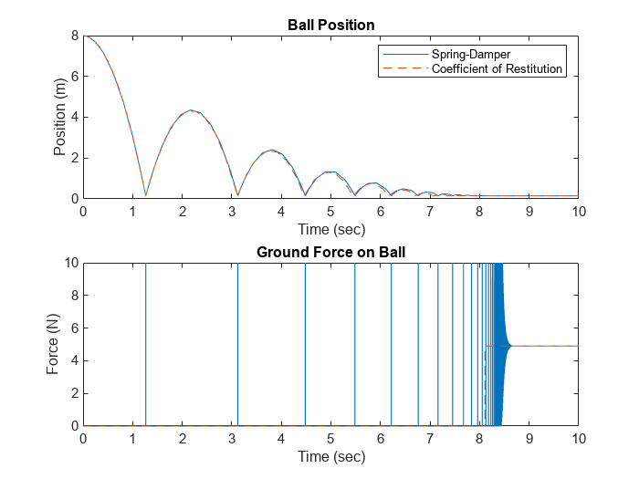
figure;

subplot(2,1,1);
plot(t_springDamper, x_springDamper)
hold on
plot(t_restitutionCoefficient, x_restitutionCoefficient, '--');
legend('Spring-Damper', 'Coefficient of Restitution')
title('Ball Position')
xlabel('Time (sec)');
ylabel('Position (m)');

subplot(2,1,2);
plot(t_springDamper, f_springDamper)
hold on
plot(t_restitutionCoefficient, f_restitutionCoefficient, '--');
ylim([0 10])
title('Ground Force on Ball')
xlabel('Time (sec)');
ylabel('Force (N)');

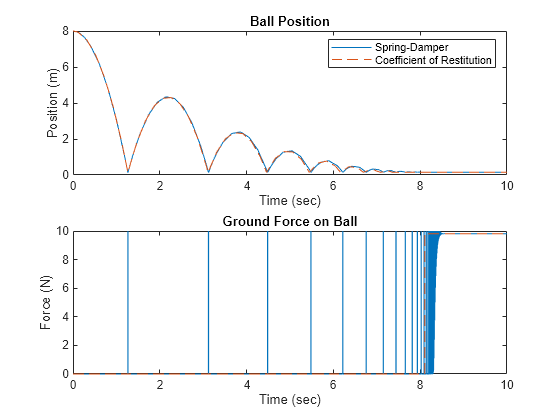
After some tuning, the two hard stop models can produce nearly identical position responses. The force responses appear different because the coefficient of restitution model does not log instantaneous impulse forces for a variable step solver. While the ball is in the air, both hard stop models exert a force of 0 N on the ball. Once the ball has come to rest, both hard stop models measure the ground's upward reaction force that counters the weight of the ball. In this scenario, the coefficient of restitution model requires much fewer time steps and has lower computational cost than the spring damper model:

num_steps_springDamper = numel(t_springDamper)

num_steps_springDamper = 3103

num_steps_restitutionCoefficient = numel(t_restitutionCoefficient)

num_steps_restitutionCoefficient = 117