Perform Controlled Charging and Discharging on Battery Module

Since R2024a

This example shows how to perform a cyclic charge and discharge profile on a battery module by using the Battery CC-CV block. At the start of the simulation, the battery module has a state of charge (SOC) of 10%. The Battery CC-CV block performs a constant-current (CC) charging until it reaches the limit cell voltage of 4.1 V specified in the Maximum cell voltage (V) parameter. The block then charges the battery with a constant-voltage (CV) profile until the module SOC reaches 90%. Finally, the block starts a CC discharging procedure and discharges the module until the SOC reaches the initial value of 10%. The charge and discharge cycle then restarts.

Model Overview

Open the controlledCharging model.

modelname = "controlledCharging";
open_system(modelname);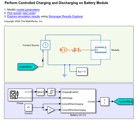

The model comprises a pre-generated Module block and a Battery CC-CV block. The Module block represents a battery module with three parallel assemblies with a gap between each parallel assembly of 0.5 mm, a detailed model resolution, and an enabled ambient thermal path. Each parallel assembly comprises four single-stacked pouch cells. Each pouch cell measures 300 mm in length, 100 mm in height, and 10 mm in thickness. For more information on how to generate the Module block, open the controlledChargingCreatelib.m file.

Run the simulation.

ssc_cntrlChrg = sim(modelname);

Simulation Results

This plot shows the current and the state of charge of the battery module during the simulation. The Battery CC-CV block charges the battery module from 10% to 90% in around 75 minutes. Then, the block discharges the battery module back to an SOC of 10% before charging it back again to 90%.

controlledChargingPlotSOC;

Results from Real-Time Simulation

This example has been tested on these platforms:

• Speedgoat™ Performance real-time target machine with an Intel® 3.5 GHz i7 multi-core CPU and 4 GB RAM.

• dSPACE® SCALEXIO LabBox with Intel® Core XEON E3-1275v3 at 3.5GHz and 4 GB RAM.

You can run this model in real time with a step size of 400 microseconds by using the Simscape local solver. For small sample rates, a task overrun might occur during the initial task execution due to a cold cache. To avoid this overrun, if the selected platform supports these options, relax the start-up behavior by specifying a limited number of task overruns or increasing the sample time of periodic tasks during the start-up phase of the real-time application.