Practical Introduction to Fatigue Analysis Using Rainflow Counting
This example describes how to perform fatigue analysis to find the total damage on a mechanical component due to cyclic stress. Fatigue is the most common mode of mechanical failure and can lead to catastrophic accidents and expensive redesigns. For this reason, fatigue life prediction and damage computation are important design aspects of mechanical systems that enable choosing materials guaranteed to last as long as required. The performance level under a certain stress history is measured by the damage, which is defined as the inverse of the fatigue life. This example uses data reported in the literature [1] and simulated stress profiles to show the workflow of fatigue analysis and damage computation.
Fatigue
Fatigue is defined as the deterioration of the structural properties of a material owing to damage caused by cyclic or fluctuating stresses. A characteristic of fatigue is the damage and loss of strength caused by cyclic stresses, with each stress much too weak to break the material [2]. The formal definition of fatigue stated by the American Society for Testing and Materials (ASTM) is as follows [3]:
The process of progressive localized permanent structural change occurring in a material subject to conditions that produce fluctuating stresses and strains at some point or points and that may culminate in cracks or complete fracture after a sufficient number of fluctuations.
The fatigue process occurs over a period of time, and the fatigue failure is often very sudden, with no obvious warning; however, the mechanisms involved may have been operating since the component or structure was first used. The fatigue process operates at local areas rather than throughout the entire component or structure. These local areas can have high stresses and strains due to external load transfer, abrupt changes in geometry, temperature differentials, residual stresses, or material imperfections. The process of fatigue involves stresses and strains that are cyclic in nature and requires more than just a sustained load. However, the magnitude and amplitude of the fluctuating stresses and strains must exceed certain material limits for the fatigue process to become critical. The ultimate cause of all fatigue failures is a crack that grows to a point such that the material can no longer tolerate the stress and suddenly fractures. The last stage of the fatigue process, known as ultimate failure or fracture, occurs when the component or structure breaks into two or more parts. In a nutshell, the fatigue process is divided into three stages:
Crack initiation
Crack propagation (crack growth)
Ultimate failure (fracture)
Fatigue is usually divided into two categories. High-cycle fatigue occurs when typically more than 10,000 cycles of low, primarily elastic stresses cause the failure to occur. Low-cycle fatigue occurs when the maximum stress exceeds the yield strength, leading to general plastic deformation.
Stress and Strain
Stress, usually denoted by , is the measure of an external force, , acting over the cross-sectional area, , of an object [4]. Stress has units of force per area. The SI unit is the pascal, abbreviated Pa: 1 Pa = 1 N/m (SI). A unit commonly used in the United States is pounds per squared inch, abbreviated psi: 1 psi = 1 lb/in. Stress can be constant- or variable-amplitude. In this example, the variable-amplitude stress profile shown below is applied to a mechanical component made of steel UNS G41300 and the damage due to this profile is computed.
load("example_fatigue_analysis_stress_history_data.mat","sg","Fs")
tg = (0:length(sg)-1)'/Fs;
plotStress(tg,sg)

Stress is often characterized by its amplitude , mean , maximum , minimum , and range . These parameters are shown in the figure below.

A half cycle is a pair of two consecutive extrema in the stress signal, going from a minimum to a maximum or from a maximum to a minimum. For a variable-amplitude stress history, the definition of one cycle is not clear and hence a reversal is often considered. Two consecutive half cycles or reversals constitute a full cycle.
When stress is applied to an object, the object deforms. Deformation is a measure of how much an object is elongated. Strain, denoted by , is the ratio between the deformation and the original length .

Stress and strain are related by a constitutive law. The more tensile stress is applied to the object, the more the object is deformed. For small values of strain, the relation between stress and strain is linear, i.e., . This linear relationship is known as Hooke's law, and the proportionality factor (often denoted by ) is known as Young's elastic modulus. The region where Hooke's law holds is referred to as the elastic region. Higher values of stress result in a non-linear stress-strain relation in the plastic region. The figure shows a typical stress-strain plot for a ductile metal like steel.

Elastic limit is the limiting value of stress up to which the material is perfectly elastic and returns to its original position when the stress is withdrawn. The yield point is the threshold after which the component material undergoes permanent plastic deformation and cannot relax back to the original shape when the stress is removed. There is an extensive plastic region that allows for the material to be drawn into wires (ductile) or beaten into sheets and easily shaped (malleable). The highest point on the graph is the ultimate tensile strength (UTS), which is the maximum stress the material undergoes before failure. At the fracture point, rupture usually occurs at the necked region with the smallest cross-sectional area because this region tolerates the least amount of stress.
Fatigue Life and Damage
The fatigue life () of a mechanical component is the number of stress cycles required to cause fracture. The fatigue life is a function of many variables, including stress level, stress state, cyclic waveform, fatigue environment, and the metallurgical condition of the material. One type of test used to measure fatigue life is crack initiation testing [5] in which mechanical components are subjected to the number of stress cycles required for a fatigue crack to initiate and to subsequently grow large enough to produce fracture. Most laboratory fatigue testing is done with axial loading, which produces only tensile and compressive stresses. The stress is usually cycled either between a maximum and a minimum tensile stress, or between a maximum tensile stress and a maximum compressive stress.
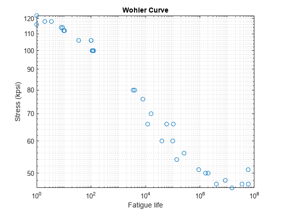
The results of fatigue crack initiation tests are usually plotted as stress amplitude against number of cycles required for ultimate failure. Whereas stress can be plotted in either a linear or a logarithmic scale, the number of cycles is plotted in a logarithmic scale. The resulting plot of the data is referred to as a Wohler curve or an S-N curve. The figure below shows a typical Wohler curve for a mechanical component. Clearly the number of cycles of stress that a metal can endure before failure increases with decreasing stress. Note that for some materials, such as titanium, the Wohler curve becomes horizontal at a certain limiting stress often referred to as the endurance limit in literature. Below this limiting stress, the component can endure an infinite number of cycles without failure.

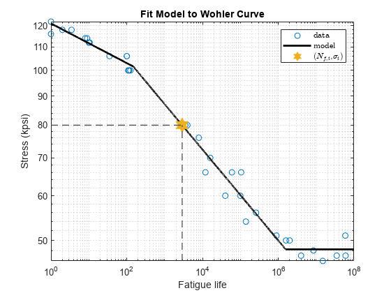
In practice, it is not feasible to obtain the fatigue for all the possible stress amplitudes in the laboratory. To save time and reduce cost, a model is often fit to the S-N data points. For many materials, a piecewise linear model can be fit to the S-N data expressed in the log-log domain. In this model, each linear piece is formulated by the Basquin expression , where is the stress amplitude, is usually referred to as the fatigue strength coefficient, is the fatigue life, and is Basquin’s exponent. If the stress amplitude is known, the corresponding fatigue life can be obtained from the piecewise linear model. The estimated fatigue life is then used to compute damage values.
As mentioned earlier, one of the objectives of this example is to compute the total damage that a mechanical component experiences due to a stress history. Towards this objective, it is important to quantify the damage first. The damage caused by one stress cycle of amplitude is defined as , where is the number of repetitions of the same stress cycle. The number can be computed from the piecewise linear model fit to the Wohler curve. Suppose that the stress profile applied to the component is composed of two blocks of stress history where each block has cycles and stress amplitude as shown in the figure.

The Palmgren-Miner rule states that the total damage due to the stress history shown above is given by . When , the component breaks. The assumption of linear damage has some shortcomings. For instance, this rule ignores the fact that the sequence and interaction of events may have major influence on fatigue life. However, this method is the simplest and most widely used approach for damage computation and fatigue life prediction [3].
Fatigue Analysis Workflow
The objective of fatigue analysis is to calculate fatigue life from a stress time series and compute the total damage. The task can be divided into two main parts:
Rainflow counting
Find total damage based on the Wohler curve and the Palmgren-Miner rule
To perform fatigue analysis, two sets of data are required: stress history and stress-life data points that are typically recorded from fatigue tests.
Rainflow Counting
Rainflow counting is used to extract the number of cycles and the stress amplitude from the stress history applied to the component. The rainflow counting consists of three steps:
Hysteresis filtering: Set a threshold and remove cycle whose contribution to the total damage is insignificant.
Peak-valley filtering: Preserve only the maximum and minimum value of the cycles and remove the points in between. Only maximum and minimum values are relevant for fatigue calculation [6].
Cycle counting using the function
rainflow.
Use the findTurningPts function to preprocess the data and prepare it for rainflow counting.
threshold = 5; % [kpsi]
[turningptsg,indg] = findTurningPts(sg,threshold);
The function denoises the stress history and removes from it inconsequential oscillations that do not contribute damage to the component. For example, the stress cycle shown in the figure leads to an insignificant closed-loop hysteresis in the stress-strain domain. After removing the hysteresis the resulting cycle will be which has some contribution to the component fracture. The task of hysteresis filtering is to remove these inconsequential cycles from the stress history data.
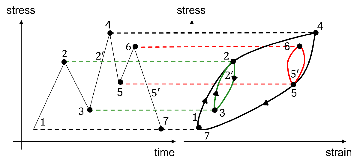
The stress-time plot results from applying the hysteresis filtering to the stress history. This figure zooms a region of the stress history to illustrate the effect of hysteresis filtering. The chosen threshold depends on the data and the material being tested. For this stress history, the threshold is set to 5 kpsi.
plotStressAndTurningPts(tg,sg,indg,turningptsg,4380,4445)

The findTurningPts function also finds the maximum and minimum values that contribute to the fatigue. Peak-valley filtering removes all data points that are not turning points. This figure shows the stress history and the turning-point series obtained at the output of the preprocessing step for a time snapshot of duration seconds.
plotStressAndTurningPts(tg,sg,indg,turningptsg,4000,4500)

After preprocessing, the next step is cycle counting. The rainflow counting method is widely used in industry to perform the counting. The turning point series obtained from the preprocessing steps is fed into the rainflow function, which returns cycle counts and stress ranges from the input signal based on the ASTM E 1049 standard [7].
rfCountg = rainflow(turningptsg,tg(indg),"ext");The rainflow function also shows the reversals as a function of time (top) and illustrates as a 2-D histogram the distribution of the found cycles as a function of stress range and mean stress (bottom). The function shows the plots if called without output arguments.
rainflow(turningptsg,tg(indg),"ext")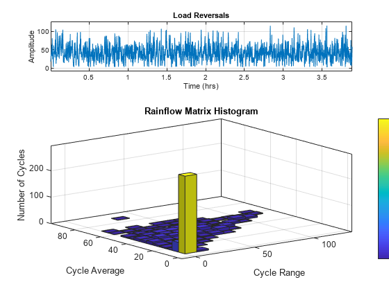
Find Damage Using Wohler Curve and Palmgren-Miner Rule
To compute the total damage, use the stress-life approach in conjunction with the rainflow counting and the Palmgren-Miner rule. In this example, we use the stress-life data from the results of axial fatigue tests on the steel UNS G41300 reported in [1]. This figure illustrates these stress-life data points.
load("example_fatigue_analysis_wohler_curve_data.mat","Nf","S")
plotWohlerCurve(Nf,S)
Next, we fit a piecewise-linear model to the stress-life data that enables the computation of the fatigue life corresponding to a certain stress without conducting the fatigue experiment. Use the piecewiseLinearFit function to perform the fit. For example, based on the derived model, the fatigue life corresponding to a stress amplitude kpsi is estimated to be . The estimateFatigueLife function carries out the estimation.
plModel = piecewiseLinearFit(Nf,S);
The fatigue life corresponding to each stress amplitude returned by the rainflow function can also be estimated by the same function estimateFatigueLife. Use the cycle counts at the output of the rainflow counting and the Palmgren-Miner rule to compute the cumulative damage due to the applied stress profile.
nig = rfCountg(:,1);
Sig = rfCountg(:,2)/2;
Nfig = estimateFatigueLife(plModel,Sig);
damageg = sum(nig./Nfig);
Since the computed total damage, is smaller than one, it can be inferred that the UNS G41300 component can tolerate the applied stress profile. This stem plot shows that the component tolerates the applied history.
cumulativeDamageStemPlot(nig,Nfig)

The same processing steps are applied to another stress history data that causes the component to break. This figure shows a small window of the stress history before and after hysteresis and P-V filtering. For this data set, the threshold is set to 10.
load("example_fatigue_analysis_stress_history_data.mat","sb")
tb = (0:length(sb)-1)'/Fs;
[turningptsb,indb] = findTurningPts(sb,10);
plotStressAndTurningPts(tb,sb,indb,turningptsb,1.91*1e4,1.955*1e4)

Now perform the rainflow counting and use the Wohler curve model and the Palmgren-Miner rule to compute the damage.
rfCountb = rainflow(turningptsb,tb(indb),"ext");
nib = rfCountb(:,1);
Sib = rfCountb(:,2)/2;
Nfib = estimateFatigueLife(plModel,Sib);
damageb = sum(nib./Nfib);
The red stem indicates that this stress history results in ultimate fracture in the component.
cumulativeDamageStemPlot(nib,Nfib)

Conclusion
This example illustrated the steps to compute the cumulative damage due to stress time series applied to a mechanical component:
Fit a theoretical model to the experimental stress-life points.
Preprocess the stress history to remove insignificant stresses leading to hysteresis and to find peaks and valleys forming stresses that contribute to damage.
Use rainflow counting to extract the cycle counts and the stress amplitudes.
Find the fatigue life corresponding to the stress amplitudes based on the theoretical Wohler curve.
Use the Palmgren-Miner rule to compute the total cumulative damage due to the stress history.
Reference
[1] Illg, W. “Fatigue Tests on Notched and Unnotched Sheet Specimens of 2024-T3 and 7075-T6 Aluminum Alloys and of SAE 4130 Steel with Special Consideration of the Life Range from 2 to 10,000 Cycles,” NACA, Hampton, VA, USA, Rep. no., NACA-TN 3866, Dec. 1956.
[2] Mouritz, A. P. Introduction to Aerospace Materials, Oxford, UK: Woodhead Publishing, 2012.
[3] Stephens, R. I., A. Fatemi, R. R. Stephens, and H. O. Fuchs, Metal Fatigue in Engineering, New York: John Wiley & Sons, 2000.
[4] Budynas, R. G., J. K. Nisbett, and J. E. Shigley, Shigley's Mechanical Engineering Design, 9th ed. New York: McGraw-Hill, 2011.
[5] Boyer, H. E., Atlas of Fatigue Curves, USA: Materials Park, OH: ASM International, 1986.
[6] Rychlik, I. "Simulation of Load Sequences from Rainflow Matrices: Markov Method," International Journal of Fatigue, vol. 18, no. 7, pp. 429–438, 1996.
[7] ASTM E1049-85, "Standard Practices for Cycle Counting in Fatigue Analysis." West Conshohocken, PA: ASTM International, 2017, https://www.astm.org/e1049-85r17.html.
Appendix
The functions listed in this section are only for use in this example. They may change or be removed in a future release.
findTurningPts
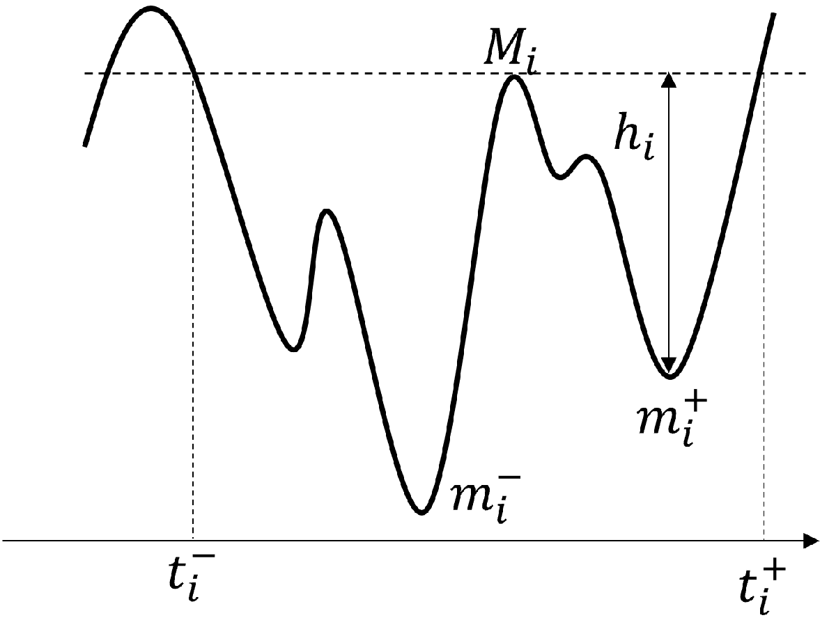
The findTurningPts function performs hysteresis and peak-valley filtering on the stress data. The inputs to the function are the stress history data, x, and a threshold for hysteresis filtering. The function pairs each local maximum in the stress history with one particular local minimum that is found as follows [6]: From a local maximum with height , the function tries to reach above in the forward or backward direction with as small a downward excursion as possible. The maximum and the minimum (which represents the smallest deviation from the maximum) form a peak-valley pair.
function [tp,ind] = findTurningPts(x,threshold)
% FINDTURNINGPTS finds turning points in signal x
%
% Reference:
% I. Rychlik, "Simulation of load sequences from rainflow matrices: Markov
% method", Int. J. Fatigue, vol. 18, no. 7m, pp. 429-438, 1996.
%
%   Copyright 2022 The MathWorks, Inc.

xLen = length(x);

% Find minimum/maximum
[~,~,zcm] = zerocrossrate(diff(x),Method="comparison",Threshold=0);
index = (1:xLen)';
zci = index(zcm);

% Make sure that there are at least two crossing points
if (length(zci) < 2)
    tp = [];
    return;
end

% Add end points
if (x(zci(1)) > x(zci(2)))
    ind = [1;zci;xLen];
else
    ind = [zci;xLen];
end

% Apply hysteresis and peak-valley filtering (a.k.a. rainflow filtering)
pvInd = hpvfilter(x(ind),threshold);
ind = ind(pvInd);

% Extract turning points
tp = x(ind);
end

function index = hpvfilter(x,h)
% HPVFILTER performs hysteresis and peak-valley filtering

% Initialization
index = [];
tStart = 1;

% Ignore the first maximum
if (x(1) > x(2))
  x(1) = [];
  tStart = 2;
end

Ntp = length(x);
Nc = floor(Ntp/2);
% Make sure that there is at least one cycle
if (Nc < 1)
    return
end

% Make sure the input sequence is a sequence of turning points
dtp = diff(x);
if any(dtp(1:end-1).*dtp(2:end) >= 0)
    error('Not a sequence of turning points.')
end

% Loop over elements of sequence
count = 0;
index = zeros(size(x));
for i = 0:Nc-2
    tiMinus = tStart+2*i;
    tiPlus = tStart+2*i+2;
    miMinus = x(2*i+1);
    miPlus = x(2*i+2+1);

    if (i ~= 0)
        j = i-1;
        while ((j >= 0) && (x(2*j+2) <= x(2*i+2)))
            if (x(2*j+1) < miMinus)
                miMinus = x(2*j+1);
                tiMinus = tStart+2*j;
            end
            j = j-1;
        end
    end

    if (miMinus >= miPlus)
        if (x(2*i+2) >= h+miMinus)
            count = count+1;
            index(count) = tiMinus;
            count = count+1;
            index(count) = tStart+2*i+1;
        end
    else
        j = i+1;
        tfFlag = false;
        while (j < Nc-1)
            tfFlag = (x(2*j+2) >= x(2*i+2));
            if tfFlag
                break
            end
            if (x(2*j+2+1) <= miPlus)
                miPlus = x(2*j+2+1);
                tiPlus = tStart+2*j+2;
            end
            j = j+1;
        end
        if tfFlag
            if (miPlus <= miMinus)
                if (x(2*i+2) >= h+miMinus)
                    count = count+1;
                    index(count) = tiMinus;
                    count = count+1;
                    index(count) = tStart+2*i+1;
                end
            elseif (x(2*i+2) >= h+miPlus)
                count = count+1;
                index(count) = tStart+2*i+1;
                count = count+1;
                index(count) = tiPlus;
            end
        elseif (x(2*i+2) >= h+miMinus)
            count = count+1;
            index(count) = tiMinus;
            count = count+1;
            index(count) = tStart+2*i+1;
        end
    end
end
index = sort(index(1:count));
end
plotStress
The plotStress function plots the stress history.
function plotStress(t,s)
plot(t,s)
title("Stress History")
xlabel("Time (sec)")
ylabel("Stress (kpsi)")
grid("minor")
end
plotStressAndTurningPts
The plotStressAndTurningPts function plots the stress history and the turning points found by the function findTurningPts. The plot focuses on a time interval starting at time ts and ending at time te.
function plotStressAndTurningPts(t,s,ind,turningpts,ts,te)
ind1 = (t >= ts) & (t <= te);
ttpts = t(ind); % time stamps of turning points
ind2 = (ttpts >= ts) & (ttpts <= te);

figure
plot(t(ind1),s(ind1))
hold on
plot(ttpts(ind2),turningpts(ind2),"-*",MarkerSize=8)
hold off
xlabel("Time (sec)")
ylabel("Stress (kpsi)")
xlim([ts,te])
legend(["Stress history" "Hysteresis & P-V filtering output"])
grid("minor")
end
plotWohlerCurve
The plotWohlerCurve function plots the Wohler curve (S-N curve).
function plotWohlerCurve(Nf,S)
loglog(Nf,S,"o")
title("Wohler Curve")
xlabel("Fatigue life")
ylabel("Stress (kpsi)")
grid("minor")
end
piecewiseLinearFit
The piecewiseLinearFit function fits a piecewise linear model to the S-N curve in log-log domain based on the Basquin relationship. It divides the fatigue life into three regions: fatigue with , , and the infinite life region with . The function returns the linear models and the region limits.
function plModel = piecewiseLinearFit(Nf,S)
x = log10(2*Nf);
y = log10(S);
% Fit piecewise linear models to three regions
% 1. Low cycle fatigue (LCF)
lcfi = Nf <= 1e3;
xlcf = x(lcfi);
ylcf = y(lcfi);
plcf = polyfit(xlcf,ylcf,1);
% 2. High cycle fatigue (HCF)
hcfi = (Nf > 1e3) & (Nf <= 1e6);
xhcf = x(hcfi);
yhcf = y(hcfi);
phcf = polyfit(xhcf,yhcf,1);
% 3. Infinite life (IL)
ili = (Nf > 1e6);
xil = x(ili);
yil = y(ili);
pil = polyfit(xil,yil,0);
% Find ending points.
Nflcf = 10^((phcf(2)-plcf(2))/(plcf(1)-phcf(1)))/2;
Nfhcf = 10^((pil(1)-phcf(2))/phcf(1))/2;
Nfil = 1e8;

% Create the model struct
plModel.plcf = plcf;
plModel.Nflcf = Nflcf;
plModel.phcf = phcf;
plModel.Nfhcf = Nfhcf;
plModel.pil = pil;
plModel.Nfil = Nfil;

% Compute stress for a range of fatigue life based on model for the sake of
% illustration
testNf = [logspace(0,log10(Nflcf),1e3), ...            % low cycle fatigue region
          logspace(log10(Nflcf),log10(Nfhcf),1e4), ... % high cycle fatigue region
          logspace(log10(Nfhcf),log10(Nfil),1e3), ...   % infinite life region
         ];
testS = computeStress(plModel,testNf);

% Fatigue life corresponding to a sample stress amplitude
Si = 80;
Nfi = estimateFatigueLife(plModel,Si);

% Plot data and piece-wise model based on Basquin relation
figure
h1 = loglog(Nf,S,"o");
hold on
h2 = loglog(testNf,testS,"-k",LineWidth=2);
h3 = loglog(Nfi,Si,"h",MarkerSize=15);
h3.MarkerFaceColor = h3.Color;
xLim = get(gca,"XLim");
yLim = get(gca,"YLim");
loglog([xLim(1) Nfi],[Si Si],"--",Color=0.3*ones(1,3),LineWidth=1)
loglog([Nfi Nfi],[yLim(1) Si],"--",Color=0.3*ones(1,3),LineWidth=1)
title("Fit Model to Wohler Curve")
xlabel("Fatigue life")
ylabel("Stress (kpsi)")
grid("minor")
legend([h1,h2,h3],["data","model","($N_{f,i}$,$\sigma_i$)"],Interpreter="latex")

end
computeStress
The computeStress function computes stress corresponding to a fatigue life given a stress-life model.
function Si = computeStress(plModel,Nfi)
Si = zeros(size(Nfi));
for i = 1:length(Nfi)
    if (Nfi(i) < plModel.Nflcf)
        % Low cycle fatigue
        Si(i) = 10.^(polyval(plModel.plcf,log10(2*Nfi(i))));
    elseif (Nfi(i) >= plModel.Nflcf && Nfi(i) < plModel.Nfhcf)
        % High cycle fatigue
        Si(i) = 10.^(polyval(plModel.phcf,log10(2*Nfi(i))));
    else
        % Infinite life
        Si(i) = 10.^(polyval(plModel.phcf,log10(2*plModel.Nfhcf)));
    end
end
end
estimateFatigueLife
The estimateFatigueLife function estimates the fatigue life corresponding to a stress amplitude given a stress-life model.
function Nfi = estimateFatigueLife(plModel,Si)
plcf = plModel.plcf;
Nflcf = plModel.Nflcf;
phcf = plModel.phcf;
Nfhcf = plModel.Nfhcf;

% Transform the stress amplitude to the log domain
logSi = log10(Si);

% Preallocate fatigue life
Nfi = NaN(size(Si));

% Loop over the stress history
for i = 1:length(Si)
    Nfi1 = 10^((logSi(i)-plcf(2))/plcf(1))/2; % low cycle fatigue
    Nfi2 = 10^((logSi(i)-phcf(2))/phcf(1))/2; % high cycle fatigue
    Nfi3 = Inf;                               % infinite life
    if (Nfi1 < Nflcf)
        Nfi(i) = Nfi1;
    elseif (Nfi2 < Nfhcf)
        Nfi(i) = Nfi2;
    else
        Nfi(i) = Nfi3;
    end
end
end
cumulativeDamageStemPlot
The cumulativeDamageStemPlot function shows the cumulative damage at each cycle using the stem function. The color of each stem is set according to the value of the damage accumulated up to the corresponding cycle. For the low-value damage, the stem color is set to a shade of green while for the high-value damage, it is set to a shade of red.
function cumulativeDamageStemPlot(ni,Nfi)
figure
L = length(ni);
damage = sum(ni./Nfi);
stem(0,NaN,"Color",[0 1 0])
title("Cumulative Damage from Palmgren-Miner Rule")
xlabel("Cycle $i$","Interpreter","latex")
ylabel("Cum. damage $D_{i} = \sum_{j=1}^{i}n_{j}/N_{f,j}$","Interpreter","latex")
set(gca,"XLim",[0 L],"YLim",[0 damage])
grid("on")
iter = unique([1:round(L/100):L,L]);
hold(gca,"on")
for i = iter
    cdi = sum(ni(1:i)./Nfi(1:i)); % cumulative damage up to cycle i
    plt = stem(i,cdi,"filled");
    setStemColor(plt,cdi,0.95)
end
end
setStemColor
The setStemColor function sets the color of the stem based on the value of the cumulative damage.
function setStemColor(hplt,cumulativeDamage,gamma)
c = lines(5);
c = c([2,3,5],:);
if (cumulativeDamage > 1)
    color = c(1,:);
else
    if (cumulativeDamage > gamma)
        c1 = c(1,:);
        c2 = c(2,:);
    else
        c1 = c(3,:);
        c2 = c(2,:);
    end
    color = zeros(1,3);
    for i = 1:3
        color(i) = c1(i)+(c2(i)-c1(i))*cumulativeDamage;
    end
end
hplt.Color = color;
end