eyeContour
Description
Use the eye contour object to store data related to a set of
contours at the specified symbol error rate (SER). The eye contours are generated from an eye
diagram.
Creation
Description
c = eyeContour(eyeObj)eyeObj
using default values.
c = eyeContour(eyeObj,Name=Value)
For example, c =
eyeContour(eyeObj,SER=1e-3,Extrapolation='None')eyeObj at
the symbol error rate 1e-3.
Input Arguments
Properties
Object Functions
eyeHeight (Mixed-Signal Blockset) | Measure vertical eye opening |
eyeWidth (Mixed-Signal Blockset) | Measure horizontal eye opening |
eyeArea (Mixed-Signal Blockset) | Measure eye area |
upperContour (Mixed-Signal Blockset) | Measure upper contour of eye diagram |
lowerContour (Mixed-Signal Blockset) | Measure lower contour of eye diagram |
closedContour (Mixed-Signal Blockset) | Measure closed contour of eye diagram |
More About
The Eye Measurement block extrapolates its 2-D histogram to a specified symbol error rate whenever it generates bathtub curves or eye contours.
During extrapolation method, the block pre-processes the data, one symbol at a time on only a 1-D slice of the said symbol. The block extrapolates the eye diagram at the specified SER value using the interpolation between the adjacent bins.
The block provides five interpolation methods (none,
linear, spline,
pchip, and makima) and two
extrapolation methods (gaussian and
dualdirac) to extrapolate data.
This image shows how the block uses interpolation methods to extrapolate data.
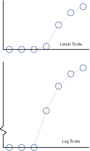
The blue dots represent the cumulative sum of the eye diagram going outward from the center of the eye. The blue dot at the x-axis value zero represents the eye opening. The dotted red line shows the interpolated samples.
The log scale image is used to create the bathtub curves. The discontinuity at the logarithmic scale is to show the zero x-axis value. The linear scale image shows how the cumulative sum of the 1-D slice of the eye looks on the same scale as the slice itself..
For example, the none extrapolation method uses a previous
neighbor interpolation of the cumulative sum an eye slice. For horizontal eye slices, the
extrapolation uses the timing origins. For vertical eye slices, the extrapolation uses the
symbol thresholds.
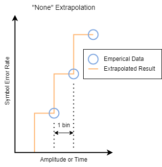
When moving outward from the center of the eye, it is a previous neighbor interpolation. When moving across the eye from one side to the other, it appears as a next neighbor interpolation that switches to a previous neighbor interpolation as you pass the center of the eye. This way, the result for a symbol error rate is a conservative estimate from the perspective of the eye opening, based on the data.
On the other hand, the dualdirac extrapolation algorithm
first fits the Dual-Dirac PDF to a column of the split histogram. Then it uses those
coefficients to calculate the inverse Dual-Dirac CDF for the specified SER(s). It is only
applicable to systems with an exponential impulse response whose time constant is on the
order of the time for one symbol, or less. The algorithm is also significantly slower that
the None extrapolation method.
This table summarizes the different extrapolation methods the block supports.
| Method | Description | Comments |
|---|---|---|
none | Uses previous neighbor interpolation of each eye slice to find the SER values. The interpolated value at any query point is the value at the previous sample grid point. |
|
dualdirac | Fits a Dual-Dirac model to each slice of the eye, then uses the fitted model to find the SER values. |
|
gaussian | Uses the Gaussian defined by the sample mean and sample standard deviation of each eye slice to find the SER values. |
|
linear | Uses linear interpolation of each eye slice to find the SER values. The interpolated value at any query point is based on linear interpolation of the values at neighboring grid points in each respective dimension. |
|
spline | Uses natural spline interpolation of the cumulative sum out from the center of each eye slice to find SER values. |
|
pchip | Uses shape-preserving piecewise cubic interpolation of each eye slice to find the SER values. The interpolated value at any query point is based on a shape-preserving piecewise cubic interpolation of the values at neighboring grid points. |
|
makima | Uses modified Akima cubic Hermite interpolation of each eye slice to find the SER values. The interpolated value at a query point is based on any piecewise function of polynomials with degree at most three. The Akima formula is modified to avoid overshoots. |
|
Version History
Introduced in R2024a
See Also
Eye Measurement (Mixed-Signal Blockset) | eyeDiagramSI (Mixed-Signal Blockset) | eyeMask (Mixed-Signal Blockset)
Topics
- Choose Extrapolation Method Based on Application (Mixed-Signal Blockset)