Resolve Partitioning Solver Simulation Issues for Simscape Driveline Models

R2026b

The Partitioning solver is a Simscape™ fixed-step, local solver that improves performance for certain models. However, when using the Partitioning solver, some Simscape Driveline™ models generate warnings, stop and generate errors, fail to initialize, or yield signal chatter due to numerical difficulties. These examples show how to eliminate errors, mitigate warnings, and reduce chatter by resolving numerical difficulties.

Resolving Issues for Blocks with Stiffness or Friction

Numerical difficulties that prevent models from simulating to completion, yield warnings, or introduce chatter are typically related to blocks that have high stiffness or friction. Simscape Driveline blocks with high stiffness or friction include clutches, belt pulleys, tires, and flexible shafts.

To resolve numerical difficulties in models that contain these blocks, use one or more of the methods:

• Adjust the solver settings.

• Remove high-priority variable redundancies.

• Unlock clutch initial conditions.

• Loosen friction-related tolerances.

• Eliminate high-stiffness blocks.

• Eliminate degrees of freedom.

Using the Partitioning Solver

When simulating models using the Partitioning solver:

1. Simulate the model by using a global variable-step solver to capture baseline results that agree with your mathematical model or empirical data.

2. Configure the local solver for a Partitioning solver simulation.

3. Run the Partitioning solver simulation. If the simulation:

   • Runs to completion — Compare the Partitioning solver simulation results to the baseline results. If the results do not agree, adjust the solver settings or model components and simulate again. For example, decrease the step size or simplify model dynamics. For more information, see Identify and Resolve System Stiffness in Simscape Models and Define Step Size and Number of Nonlinear Iterations for Simscape Real-Time Simulation.

     Repeat until the simulation returns results that agree with the baseline results.

   • Fails to simulate to completion due to numerical issues — Resolve the issues by applying one or more of the methods listed in Resolving Issues for Blocks with Stiffness or Friction. Rerun the simulation. Repeat until the simulation runs to completion, then compare the results to the baseline results. If the results do not agree, adjust the solver settings or model components and rerun the simulation. Repeat until the Partitioning solver simulation returns results that agree with the baseline results.

Diagnose Unexpected Simulation Behavior Due to Nonlinearities

This example uses a model of a helicopter taking off to show how to diagnose a numerical issue caused by a nonlinearity. The model uses a Translational Hard Stop block to represent the interaction of the helicopter chassis with the ground. When the helicopter takes off, the block implements smoothing to transition away from a position of zero. The partitioning solver produces unexpected results because of this smoothed transition.

1. Open the model. At the MATLAB^® command prompt, enter:

   See Code

   openExample('sdl/HelicopterTransmissionExample')

   

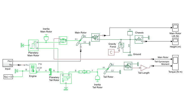
   Note that the automatic solver selection is ode23t. This is a variable-step solver.

2. Inspect the Solver Configuration block settings

   See Code

   model = 'HelicopterTransmission';
   solvConfig = 'Solver Configuration';
   solvConfigPath = [model,'/',solvConfig];
   open_system(solvConfigPath)

   Note that Use local solver is off. This means that the simulation uses a global solver.

3. Generate baseline results from the variable-step, global solver and open the Scope block.

   See Code

   sim(model)
   scope = 'Main Rotor Lift (N)';
   scopePath = [model,'/',scope];
   open_system(scopePath)
   

   

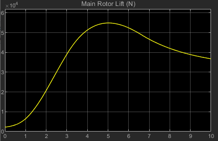
4. Configure the model to use the partitioning solver. In the Solver Configuration block settings, select Use local solver.

   See Code

   open_system(solvConfigPath)
   set_param(solvConfigPath,...
       'UseLocalSolver','on',...
       'DoFixedCost','on')

   When you select Use local solver, the block enables related parameters. The default parameter settings are:

   1. Solver type — Partitioning

   2. Sample time — 0.05

   3. Partition method — Robust simulation

   4. Partition storage method — Exhaustive

   5. Use fixed-cost runtime consistency iterations — on

   6. Nonlinear iterations — 3

5. Simulate the model.

   See Code

   sim(model)
   open_system(scopePath)
   

   

   The simulation runs to completion, but it generates unexpected results.

6. To diagnose this behavior, reduce the simulation sample time. Set Sample time to 0.01 and run the simulation.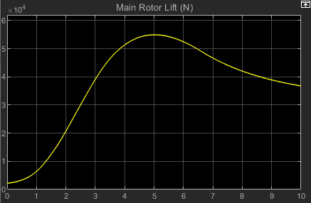

   See Code

   open_system(solvConfigPath)
   set_param(solvConfigPath,'LocalSolverSampleTime','0.01')
   
   sim(model)
   open_system(scopePath)

   

   The partitioning solver results now reflect the baseline results. This confirms that the model is valid and is generated unexpected results for numerical reasons.

7. To diagnose the numerical issue, examine the results in the Simscape Results Explorer. Compare Chassis.f and Translational_Hard_Stop.f to observe the fast dynamics that affect the system.

   See Code

   sscexplore(simlog_sdl_transmission_helicopter_base);

   

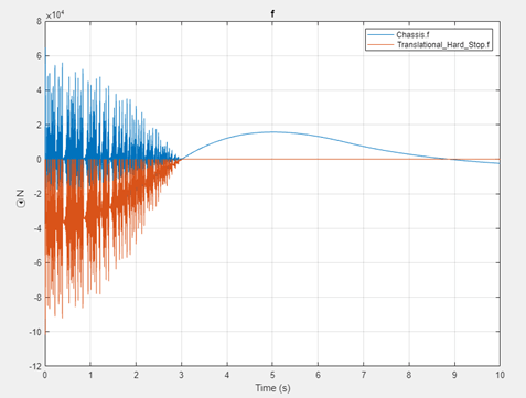
   The force variables both show excessive noise at the beginning of the simulation, when the helicopter takes off. You can use the Statistics Viewer tool to learn more about the nature of the problem. The figure shows Translational_Hard_Stop.f is in a partition by itself.

   

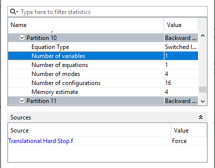
   Translational_Hard_Stop.x is in a different partition because the force and position relationship is nonlinear in the current configuration of the Translational Hard Stop block. The dependency on Translational_Hard_Stop.x causes Chassis.f to also behave unexpectedly.

8. To generate accurate results using a 0.05 time step, you must remove the nonlinearity. Because the Translational Hard Stop block in the model uses the Stiffness and damping applied smoothly through transition region, damped rebound setting by default, the block implements smoothing near zero, when the helicopter takes off. This smoothing introduces a nonlinearity that the partitioning solver resolves by splitting the force variables and position variables into different partitions.

   Choose a setting that avoids nonlinearities. Set Hard stop model to Full stiffness and damping applied at bounds, damped rebound and reset the solver sample time to its original value. Finally, run the simulation again and open the Scope block to view the results.

   See Code

   hardStop = 'Translational Hard Stop';
   hardStopPath = [model,'/',hardStop];
   open_system(hardStopPath)
   set_param(hardStopPath,'model','simscape.enum.hardstop.fulldamped')
   
   open_system(solvConfigPath)
   set_param(solvConfigPath,'LocalSolverSampleTime','0.05')
   
   sim(model)
   open_system(scopePath)

   Removing the smoothing from the Translational Hard Stop block causes the simulation to generate the correct results using the original sample time.

   

9. Confirm that these actions remove the noise in the system. Open the Simscape Results Explorer and compare Chassis.f and Translational_Hard_Stop.f again.

   See Code

   sscexplore(simlog_sdl_transmission_helicopter_base);

   

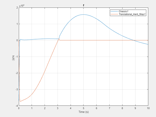
   Noise is not present in the updated solver configuration for both Chassis.f and Translational_Hard_Stop.f.

Resolve Chatter Due to Stiffness

This example also shows how to resolve numerical difficulties that yield chatter in Simscape Driveline simulations that use the Partitioning solver. In this case, the chatter is caused by stiffness. A stiff model is one that contains both fast and slow dynamics.

1. Open the model with block. At the MATLAB command prompt, enter:

   openExample('sdl/VehicleWithDualClutchTransmissionExample')
   model = 'VehicleWithDualClutchTransmission';
   

   

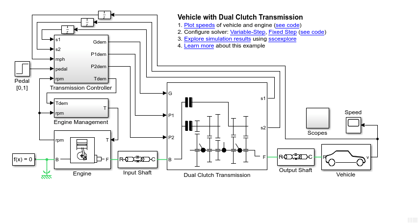
   The model is configured for a variable-step simulation that uses the global solver. Data logging is enabled only for the signal that contains the gear state data.

2. Configure the model for data logging. For this example, tire slip is the data of interest and logging additional data increases the computational cost of simulation. Enable data logging for tire slip and disable data logging for the gear state.

   1. In the Vehicle subsystem, the Tire LF Tire (Magic Formula) block represents the left-front tire of the vehicle. The Tire LF S port, which transmits the tire slip data, is a physical signal port. You can log physical signal data using Simulink^® data logging. The destination for the signal is the Tire slip Scope block, which is in the Scopes subsystem.

      1. Open the Scopes subsystem.

      2. The tire slip data is in the signal that the FrontSlip From block transmits to the Tire slip Scope block. Select the signal, and in the Simulink toolstrip, on the Signal tab, click the arrow on the right side of the Monitor section. In the Signal Monitoring category, click Log Signals.

      See Code

      %% Enable Tire Slip Data Logging
      % Enable Logging for Front Left Tire Slip Signal
      
      % Define Scope Subsystem and path
      scopesSS = 'Scopes';
      scopesSSPath = [model,'/',scopesSS];
      
      %% Define Front Slip From Tag Signal
      fromTireLFLogSlip1 = 'From8';
      fromTireLFLogSlip1Path = [scopesSSPath,'/',fromTireLFLogSlip1];
      
      %% Enable the Front Slip From Tag Signal for   
      % Simulink(TM) data logging and viewing with the Simulation Data Inspector
      
      fromTireLFLogSlip1PortHandles = get_param(fromTireLFLogSlip1Path,...
          'PortHandles');
      fromTireLFLogSlip1Outport = fromTireLFLogSlip1PortHandles.Outport;
      set_param(fromTireLFLogSlip1Outport,'DataLogging','on')
      

   2. In the Transmission Controller subsystem, in the Shift state subsystem, the z3 Unit Delay block transmits the gear state.

      1. Open the Transmission Controller subsystem.

      2. Open the Shift state subsystem.

      3. The Gear state G subsystem transmits the gear state to a Unit Delay block, which, in turn, transmits the data to the Gear state Outport block. The signal that connects the Unit Delay block to the Gear state Outport block is marked for data logging. Select the signal, and in the Simulink toolstrip, on the Signal tab, click the arrow on the right side of the Monitor section. In the Signal Monitoring category, click Log Signals.

      See Code

      %% Disable Gear State Data Logging
      
      % Define Transmission Controller Subsystem and Path
      transCntrl = 'Transmission Controller';
      transCntrlPath = [model,'/',transCntrl];
      
      % Define Shift State Subsystem and path
      shiftState = 'Shift state';
      shiftStatePath = [transCntrlPath,'/',shiftState];
      
      % Define Unit Delay block and path
      unitDelay = 'z3';
      unitDelayPath = [shiftStatePath,'/',unitDelay];
      
      % Disable Unit Delay block signal logging
      unitDelayPortHandles = get_param(unitDelayPath,'PortHandles');
      unitDelayOutport = unitDelayPortHandles.Outport;
      set_param(unitDelayOutport,'DataLogging','off')
      

3. Obtain and examine the baseline results. Simulate using the global variable-step solver and review the results in the Simulation Data Inspector.

   1. Run the simulation. In the Simulink toolstrip, on the Simulation tab, in the Simulate section, click Run.

      See Code

      %% Simulate the Model
      sim(model)
      

   2. Open the Simulation Data Inspector. In the Simulink toolstrip, on the Simulation tab, click the arrow on the right side of the Review Results section, and, in the Signal Logging Results category, click Signal Logging Results. To inspect the tire slip data, select the From8:1 check box.

      See Code

      %% Examine Baseline Results in the Simulation Data Inspector
      
      % Define Baseline Run
      runIDs = Simulink.sdi.getAllRunIDs;
      baselineRunID = runIDs(end);
      baselineRun = Simulink.sdi.getRun(baselineRunID);
      baselineRunTireLFSlip = baselineRun.getSignalByIndex(1);
      
      % Set Line Color
      baselineRunTireLFSlip.LineColor = [0    0.4470    0.7410];
      
      % Select Signal (From8:1) Check Box
      baselineRunTireLFSlip.Checked = true;
      
      %% Open Simulation Data Inspector
      Simulink.sdi.view
      

   

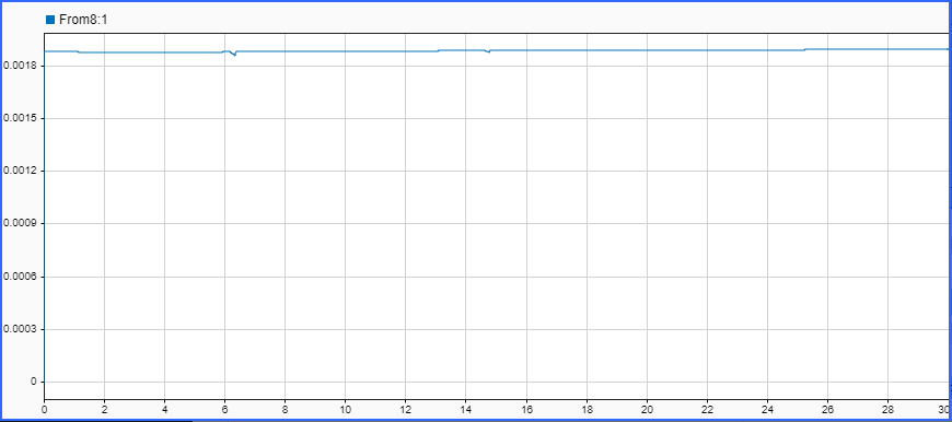
4. Configure the local solver for fixed-step simulation using the Partitioning solver.

   1. In the model, open the Solver Configuration block settings.

   2. Select the Use local solver check box.

   See Code

   %% Define the Solver Configuration Block and Path
   solvConfig = 'Solver Configuration';
   solvConfigPath = [model,'/',solvConfig];
   
   %% Configure the Solver Configuration Block
   set_param(solvConfigPath,...
       'UseLocalSolver','on',...
       'DoFixedCost','on')
   

5. Simulate using the Partitioning solver.

   See Code

   %% Simulate the Model
   sim(model)
   

   The simulation runs to completion, but generates a warning.

   Warning: Simscape succeeded in finding consistent states with which to start 
   the simulation, but the states found may deviate from requested initial conditions.

6. Compare the baseline and Partitioning solver results in the Simulation Data Inspector.

   1. Open the Simulation Data Inspector.

   2. In the top, left pane, select Compare.

   3. Configure the comparison. In the top, right pane:

      1. On the right side of the Baseline setting, click the down arrow and select Run 1: sdl_vehicle_clutch.

      2. On the right side of the Compare to setting, click the down arrow and select Run 2: sdl_vehicle_clutch.

      3. Click Compare.

   4. To change the Partitioning solver results line color, in the Properties pane, in the Compare to column, click the colored Line, select a different color, such as yellow, and then click Set.

   See Code

   %% Compare Partioning Solver Run 1 to Baseline Run
   % Open Simulation Data Inspector
   Simulink.sdi.view
   
   % Define Partitioning Solver Run 1
   runIDs = Simulink.sdi.getAllRunIDs;
   pSolverRun1ID = runIDs(end);
   pSolverRun1 = Simulink.sdi.getRun(pSolverRun1ID);
   psolverRun1TireLFSlip = pSolverRun1.getSignalByIndex(1);
   
   % Select From8:1 Check Box
   % psolverRun1TireLFSlip.Checked = true;
   
   % Set Line Color
   psolverRun1TireLFSlip.LineColor = [0.9294    0.6941    .1255];
   
   % Compare Runs
   compBaselinePartition1 = Simulink.sdi.compareRuns(baselineRunID,...
       pSolverRun1ID);
   

   

   The results from the Partitioning solver simulation contain significant chatter.

7. Chatter in the front tire slip is due to the parameters specified for the Tire (Magic Formula) block. To resolve the signal chatter and the initial condition warning, simplify the tire dynamics:

   1. Open the Vehicle subsystem.

   2. Open the Tire LF block settings.

   3. In the Dynamics settings, set Inertia to No Inertia.

   4. Using the same process, omit the inertia for the Tire RF, Tire LR, and Tire RR blocks.

   See Code

   %% Resolve Chatter
   % Simplify Tire Dynamics by Removing Inertia
   
   % Define Vehicle Subsystem and Paths
   vehicle = 'Vehicle';
   vehiclePath = [model,'/',vehicle];
   
   %% Define Tire Blocks and Paths and Omit Tire Inertia
   %% Define Tire LF
   tireLF = 'Tire LF';
   tireLFPath = [vehiclePath,'/',tireLF];
   
   %% Set Tire LF Settings Dymamics > Inertia to "No inertia"
   set_param(tireLFPath, 'model_inertia', '0')
   
   %% Omit Inertia from Tire RF, LR, RR Blocks
   
   % Tire RF
   tireRF = 'Tire RF';
   tireRFPath = [vehiclePath,'/',tireRF];
   set_param(tireRFPath, 'model_inertia', '0')
   
   % Tire LR
   tireLR = 'Tire LR';
   tireLRPath = [vehiclePath,'/',tireLR];
   set_param(tireLRPath, 'model_inertia', '0')
   
   % Tire RR 
   tireRR = 'Tire RR';
   tireRRPath = [vehiclePath,'/',tireRR];
   set_param(tireRRPath, 'model_inertia', '0')
   

8. Simulate and then examine and compare the results in the Simulation Data Inspector.

   1. Run the simulation.

      See Code

      sim(model)
      

      The simulation runs to completion, and does not generate any initial condition warnings.

   2. Open the Simulation Data Inspector and compare the results from the Partitioning solver fixed-step simulation to the baseline results from the variable-step simulation. To configure the comparison, in the top, right pane:

      1. On the right side of the Baseline setting, click the down arrow and select Run 1: sdl_vehicle_clutch.

      2. On the right side of the Compare to setting, click the down arrow and select Run 3: sdl_vehicle_clutch.

      3. Click Compare.

   See Code

   %% Open the Simulation Data Inspector
   Simulink.sdi.view
   
   %% Define the baseline run and select the From tag check box
   runIDs = Simulink.sdi.getAllRunIDs;
   pSolverRun2ID = runIDs(end);
   pSolverRun2 = Simulink.sdi.getRun(pSolverRun1ID);
   psolverRun2TireLFSlip = pSolverRun1.getSignalByIndex(1);
   psolverRun2TireLFSlip.LineColor = [0.9294    0.6941    .1255];
   psolverRun2TireLFSlip.Checked = true;
   
   % Compare the results
   compBaselinePartition2 = Simulink.sdi.compareRuns(baselineRunID,...
       pSolverRun2ID);

   

   The results from the Partitioning solver simulation no longer contain significant chatter and are much more similar to the baseline results.