Robust Tuning of Positioning System
This example shows how to take into account model uncertainty when tuning a motion control system.
Background
This example refines the design discussed in the "Tuning of a Digital Motion Control System" example. The positioning system under consideration is shown below.

Figure 1: Digital motion control hardware
A physical model of the plant is shown in the "Plant Model" block of the Simulink model rct_dmcNotch:

Figure 2: Equations of motion
In the earlier example, we tuned the controller using "crisp" values for the physical parameters  . In reality, these parameter values are only known approximately and may vary over time. Because the resulting model discrepancies can adversely affect controller performance, we need to account for parameter uncertainty during tuning to ensure robust performance over the range of possible parameter values. This process is called robust tuning.
Modeling Uncertainty
Assume 25% uncertainty on the value of the stiffness  , and 50% uncertainty on the values of the damping coefficients
  . Use the
 ureal object to model these uncertainty ranges.
b1 = ureal('b1',1e-6,'Percent',50);
b2 = ureal('b2',1e-6,'Percent',50);
b12 = ureal('b12',5e-7,'Percent',50);
k = ureal('k',0.013,'Percent',25);
Using the equations of motion in Figure 2, we can derive a state-space model G of the plant expressed in terms of  :
:
J1 = 1e-6; J2 = 1.15e-7;
A = [0 1 0 0; -k/J1 -(b1+b12)/J1 k/J1 b12/J1; 0 0 0 1; k/J2 b12/J2 -k/J2 -(b2+b12)/J2 ];
B = [ 0; 1/J1 ; 0	; 0 ];
C = [ 0  0  1  0 ];
D  = 0;
G = ss(A,B,C,D,'InputName','u','OutputName','pos_L')
Uncertain continuous-time state-space model with 1 outputs, 1 inputs, 4 states.
The model uncertainty consists of the following blocks:
  b1: Uncertain real, nominal = 1e-06, variability = [-50,50]%, 1 occurrences
  b12: Uncertain real, nominal = 5e-07, variability = [-50,50]%, 1 occurrences
  b2: Uncertain real, nominal = 1e-06, variability = [-50,50]%, 1 occurrences
  k: Uncertain real, nominal = 0.013, variability = [-25,25]%, 1 occurrences

Type "G.NominalValue" to see the nominal value and "G.Uncertainty" to interact with the uncertain elements.
Note that the resulting model G depends on the uncertain parameters  . To assess how uncertainty impacts the plant, plot its Bode response for different values of
  . By default, the
 bode function uses 20 randomly selected values in the uncertainty range. Note that both the damping and natural frequency of the main resonance are affected.
rng(0), bode(G,{1e0,1e4})

Nominal Tuning
To compare nominal and robust tuning, we first repeat the nominal design done in the "Tuning of a Digital Motion Control System" example. The controller consists of a lead-lag compensator and a notch filter:
% Tunable lead-lag
LL = tunableTF('LL',1,1);

% Tunable notch (s^2+2*zeta1*wn*s+wn^2)/(s^2+2*zeta2*wn*s+wn^2)
wn = realp('wn',300);   wn.Minimum = 300;
zeta1 = realp('zeta1',1);   zeta1.Minimum = 0;   zeta1.Maximum = 1;
zeta2 = realp('zeta2',1);   zeta2.Minimum = 0;   zeta2.Maximum = 1;
N = tf([1 2*zeta1*wn wn^2],[1 2*zeta2*wn wn^2]);

% Overall controller
C = N * LL;
Use feedback to build a closed-loop model T0 that includes both the tunable and uncertain elements.
AP = AnalysisPoint('u',1);  % to access control signal u
T0 = feedback(G*AP*C,1);
T0.InputName = 'ref'
Generalized continuous-time state-space model with 1 outputs, 1 inputs, 7 states, and the following blocks:
  LL: Tunable SISO transfer function, 1 zeros, 1 poles, 1 occurrences.
  b1: Uncertain real, nominal = 1e-06, variability = [-50,50]%, 1 occurrences
  b12: Uncertain real, nominal = 5e-07, variability = [-50,50]%, 1 occurrences
  b2: Uncertain real, nominal = 1e-06, variability = [-50,50]%, 1 occurrences
  k: Uncertain real, nominal = 0.013, variability = [-25,25]%, 1 occurrences
  u: Analysis point, 1 channels, 1 occurrences.
  wn: Scalar parameter, 6 occurrences.
  zeta1: Scalar parameter, 1 occurrences.
  zeta2: Scalar parameter, 1 occurrences.

Type "ss(T0)" to see the current value and "T0.Blocks" to interact with the blocks.
The main tuning goals are:
Open-loop bandwidth of 50 rad/s
Gain and phase stability margins of at least 7.6 dB and 45 degrees
To prevent fast dynamics, we further limit the natural frequency of closed-loop poles.
s = tf('s');
R1 = TuningGoal.LoopShape('u',50/s);
R2 = TuningGoal.Margins('u',7.6,45);
R3 = TuningGoal.Poles('u',0,0,1e3);   % natural frequency < 1000
Now tune the controller parameters for the nominal plant subject to the three tuning goals.
T = systune(getNominal(T0),[R1 R2 R3]);
Final: Soft = 0.907, Hard = -Inf, Iterations = 100
The final value indicates that all design objectives were nominally met and the closed-loop response looks good.
step(T), title('Nominal closed-loop response')

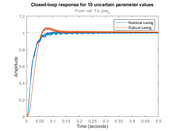
How robust is this design? To find out, update the uncertain closed-loop model T0 with the nominally tuned controller parameters and plot the closed-loop step response for 10 random samples of the uncertain parameters.
Tnom = setBlockValue(T0,T);       % update T0 with tuned valued from systune
[Tnom10,S10] = usample(Tnom,10);  % sample the uncertainty
step(Tnom10,0.5)
title('Closed-loop response for 10 uncertain parameter values')

This plot reveals significant oscillations when moving away from the nominal values of  .
.
Robust Tuning
Next re-tune the controller using the uncertain closed-loop model T0 instead of its nominal value. This instructs systune to enforce the tuning goals over the entire uncertainty range.
[Trob,fSoft,~,Info] = systune(T0,[R1 R2 R3]);
Soft: [0.907,19.3], Hard: [-Inf,-Inf], Iterations = 100
Soft: [1.02,3.75], Hard: [-Inf,-Inf], Iterations = 49
Soft: [1.25,1.85], Hard: [-Inf,-Inf], Iterations = 43
Soft: [1.26,1.26], Hard: [-Inf,-Inf], Iterations = 29
Final: Soft = 1.26, Hard = -Inf, Iterations = 221
The achieved performance is a bit worse than for nominal tuning, which is expected given the additional robustness constraint. Compare performance with the nominal design.
Trob10 = usubs(Trob,S10); % use the same 10 uncertainty samples
step(Tnom10,Trob10,0.5)
title('Closed-loop response for 10 uncertain parameter values')
legend('Nominal tuning','Robust tuning');

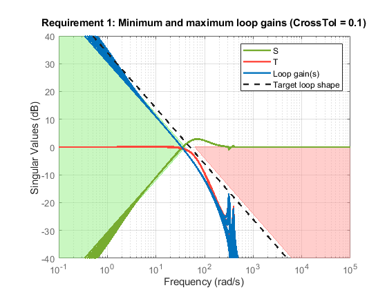
The robust design has more overshoot but is largely free of oscillations. Verify that the plant resonance is robustly attenuated.
viewGoal(R1,Trob)

Finally, compare the nominal and robust controllers.
Cnom = setBlockValue(C,Tnom);
Crob = setBlockValue(C,Trob);
bode(Cnom,Crob), grid, title('Controller')
legend('Nominal tuning','Robust tuning');

Not surprisingly, the robust controller uses a wider and deeper notch to accommodate the damping and natural frequency variations in the plant resonance. Using systune's robust tuning capability, you can automatically position and calibrate the notch to best compensate for such variability.
Worst-Case Analysis
The fourth output argument of systune contains information about worst-case combinations of uncertain parameters. These combinations are listed in decreasing order of severity.
WCU = Info.wcPert
WCU =

  5×1 struct array with fields:

    b1
    b12
    b2
    k
WCU(1) % worst-overall combination
ans =

  struct with fields:

     b1: 5.0000e-07
    b12: 7.5000e-07
     b2: 5.0000e-07
      k: 0.0163
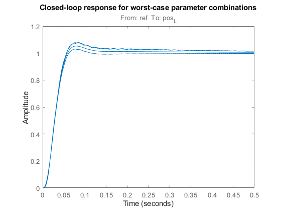
To analyze the worst-case responses, substitute these parameter values in the closed-loop model Trob.
Twc = usubs(Trob,WCU);
step(Twc,0.5)
title('Closed-loop response for worst-case parameter combinations')
